

Introduction
Literature Review
Research status of two-dimensional interpolation
Research status of three-dimensional interpolation
Methodology
Kriging Method
Implementation steps of ordinary Kriging
Volume Calculation
Case Study
Case introduction
Result and Discussions
Conclusions
Introduction
At present, there are many methods to measure earthwork, but there are few methods with relatively high accuracy, and the error of earthwork is difficult to control. In this case, how to improve the accuracy of earthwork calculation is of great significance to the control of Engineering economy. With the continuous increase of construction projects, earthwork projects of various sizes will be produced, and earthwork budget estimates also account for a considerable proportion. Therefore, the study of earthwork measurement will directly affect the investment budget and cost of the project, which has great reference value for regulating the cost and progress of the project. Using effective methods to measure and calculate the amount of excavated and filled earth, and processing the acquired data, we can get the amount of excavated and filled earth data. With accurate amount of earth, we can reasonably allocate earthwork, control the cost of the project, and speed up the progress of the project. It is of great significance to improve the quality of the project.
Spatial interpolation is an interpolation method for estimating spatial data values of unknown regions by spatial data of known sampling points [1]. Spatial interpolation is based on the hypothesis of "the first law of geography": the closer the spatial position is, the greater the likelihood of having similar characteristics; the farther the distance is, the less likely the likelihood of having similar characteristics; that is, there is spatial correlation between geological attributes [2]. Li and Heap [3] summarized and compared the mathematical methods, interpolation effects, influencing factors and using conditions of deterministic interpolation, spatial statistical interpolation and comprehensive interpolation methods.
There are many kinds of spatial interpolation methods, each of which has its applicable scope, algorithms, advantages and disadvantages [4]. Compared with other methods, spatial statistical method, namely geostatistical method, not only considers the spatial correlation of objects, but also gives the estimation error of prediction points. Kriging is one of the main research contents of geostatistics. It is named after Kriging, a mining engineer in South Africa. It was developed by Matheron, a French geostatistician [5]. Kriging method calculates the weight by introducing a variation function (also known as variation function) with distance as independent variable, and calculates the estimated value of space point by linear combination of sampling point and weight matrix. In this paper, the research status of Kriging method is mainly discussed from two aspects of two-dimensional interpolation and three-dimensional interpolation.
Literature Review
There are a number of interpolation method such as spline interpolation, linear interpolation, minimum curvature interpolation, natural neighbor point interpolation, and Kriging method. On one hand it is necessary to undergo the history of interpolation for better understand the Kriging method, on the other hand, it takes too much of space to describe the detail. This paper, thus, focused on the explanation of Kriging method in both two- and three- dimensional interpolation.
Research status of two-dimensional interpolation
In terms of two-dimensional interpolation, Hengl [6] proposed a framework of spatial prediction method based on regression Kriging. Combining DEM, topographic gradient and soil unit map, the spatial structure of soil variables and residuals was modeled by variogram fitting, and the soil thickness was visualized by interpolation. Goovaerts et al. [7] proposed a method to obtain spatial continuous distribution of soil properties by combining point and surface data with spatial interpolation. These usual interpolation assumptions assume that the data are isotropic. Space field is regarded as homogeneous space. Scholars at home and abroad have also studied two-dimensional Kriging interpolation considering anisotropy.
Geological space is a complex three-dimensional space field. In order to interpolate and reconstruct the three-dimensional space, the three-dimensional space value is transformed into a combination of two-dimensional interpolation and one-dimensional space. The three-dimensional space is divided into several horizontal layers in the vertical direction, namely two-dimensional plane. First, the horizontal projection points of observation points are interpolated in a certain way in the vertical direction, and then the interpolation points of each layer are used again. Two-dimensional Kriging interpolation is used to obtain three-dimensional space fields [8]. Li Xiaojun et al. [9] numbered the strata according to stratigraphic sequence, constructed a three-dimensional stratigraphic model from borehole information, and then used Kriging method to predict the boundary points of each stratum in the whole three-dimensional strata, so as to obtain three-dimensional digital strata.
Kriging spatial interpolation is a local interpolation algorithm. It is necessary to obtain the range parameters of the sampling point according to the variation function. In the range of variation, the neighborhood search radius of the interpolation point is determined by searching its neighborhood points as known points. Because of the anisotropy of geological space and the different range of observation data in different directions, neighborhood search is an indispensable part of spatial interpolation calculation. The search neighborhood of Kriging interpolation is generally divided into fixed radius method and fixed-point number method and quadrant search method. Fixed radius method is centered on the point to be interpolated and the radius is fixed distance. All points falling within the fixed distance range are taken as participating calculation points. This method is simple and easy to implement, but when the distribution of sample points is not uniform, there will be too many or too many search points. Too few of them affect the interpolation accuracy. Fixed-point method is to determine the number of neighborhood points and select the nearest point to be interpolated as the known point. The algorithm is simple, but the uneven distribution of sample points may lead to extrapolation. Quadrant search method divides the region into several objects, each quadrant limits the maximum number of selected points. Neighborhood points in the same quadrant can only be selected according to distance.
Research status of three-dimensional interpolation
The research status of three-dimensional interpolation is very mature, but it cannot reflect the distribution of three-dimensional geological phenomena in real space. Researchers and scholars have studied and explored three-dimensional spatial interpolation methods, most of which are based on two-dimensional spatial interpolation methods and three-dimensional extension on models. Li et al. [10] proposed a finite element interpolation method for three-dimensional function interpolation model, which divides Delaunay tetrahedron into three-dimensional space. The sum of the product of the attribute values of four nodes and the weight of the three-dimensional shape function of nodes is the interpolation result of any point in the tetrahedron. This kind of three-dimensional proximity interpolation method is suitable for observation data with catastrophe values, and has good adaptability. However, only interpolation based on geometric structure cannot reflect the structural change characteristics of three-dimensional geological space. Lafuerza et al. [11] studied the uneven distribution of sampling points in the delta region. First, they divided the three-dimensional regular grids into three-dimensional grids, and then used the extended three-dimensional minimum tension grid bicubic spline algorithm to interpolate the attributes such as vertex drag.
Three-dimensional Kriging spatial interpolation is an extension of three-dimensional space, which has the characteristics of optimal linear unbiased estimation. It can also take full account of the spatial structure characteristics to make the results of three-dimensional spatial estimation more accurate [12]. Regardless of the anisotropy of space field, the variogram is constructed directly from known points in unit space and fitted by some method. The attributes of unknown points are estimated by Kriging interpolation [13]. Considering the variation characteristics of spatial field anisotropy, variograms are obtained in X, Y and Z directions respectively, and then integrated into comprehensive variograms for three-dimensional Kriging interpolation [14, 15]. Pan Mao's team proposed a nested method for the structural analysis of three-dimensional anisotropic variograms. Through the transformation of spatial coordinate bases, the radial and axial variograms were combined to describe the variation law of variograms in three-dimensional space. Using unbiased Kriging algorithm, a new variogram is proposed and combined with curve fitting method. The interpolation of point cloud data shows that the combination of the two methods has greatly improved the interpolation effect.
Methodology
Kriging Method
Kriging method, also known as local estimation, plays an important role in the field of geostatistics [16]. This method is based on the analysis of variation function and structure. It estimates unbiased optimal values of variables in a certain range. Kriging is a spatial estimation technology created by Krige, a South African geologist. It was originally applied to the estimation of geological reserves. Professor Sacks said that Kriging theory was further popularized and applied in the fields of geology, hydrology and meteorology [17, 18]. This method mainly comes from the prediction of mining species. It is the best possible prediction of the average grade of the ore block by analyzing all kinds of ore samples in a certain area. In the field of mathematics, it is a kind of method to find the best value and unbiased interpolation estimator. This method gives the sample value a certain weight coefficient and uses weighted average after fully analyzing various factors. The method is used to obtain the final result. The factors mentioned here include the sample size, the relationship between the sample size and the segment to be estimated, the spatial structure of the variable, and so on.
Kriging method can maximize the use of the obtained information. By considering the relationship between the estimated point and the known sample points and the relationship between each sample point, the information of a certain point can be obtained. At the same time, the distribution characteristics of known values [19] are used. This method is composed of the following parts, including ordinary Kriging, indicator Kriging, etc. [6].
The Kriging classes currently used generally include the following categories: simple and common methods belong to the category of linear stationary geostatistics, i.e. linear unbiased estimators with predicted values of known values; if the variables meet the second-order stationary or intrinsic assumptions, common methods can be used; if the data used are not stable and there are large fluctuations, pan-Kriging method can be used. In 2008, this method belongs to the category of linear and non-stationary geostatistics, and the predicted values are the same as above. If there are two or more variables and the nature of synergistic regionalization appears, the synergetic method is the best method, and it also belongs to multivariate statistics. It expands the most suitable estimation method from one attribute to multi-regional synergistic attributes and analyses the correlation and space between variables. The relationship improves the estimation accuracy of principal variables. When using logarithmic Kriging method, it usually obeys normal distribution; indicates Kriging to be used for spatial prediction of category variables, such as pollutant risk and decision analysis, indicates Kriging to convert the original data into (0,1) values, and then estimates with this method, which does not involve parameters, but is also the key method in statistics; and uses non-linear estimators to obtain the available data. The disjunctive Kriging method can avoid the disadvantage of inaccurate estimation of regionalized variables when the numerical dispersion of regionalized variables is too large and that regionalized variables can only be estimated and the value of regionalized variables cannot be estimated. The effect of probability method is basically the same as that of indicator method, which does not use the transformed indicator form, but uses the standard order to replace the original data. Instead, when probability method is introduced into synergy method, its application effect is better than indicator method; for those cases where there is no large amount of data, there is no regularity and accuracy is not required excessively, random method is the most suitable.
Implementation steps of ordinary Kriging
(1) To calculate the distance between known data points, the first step of using ordinary Kriging algorithm is to construct the corresponding coefficient proof and matrix formula 18, which is to seek variation Cij and Ci0. The variation function is only related to the distance between sample points, but not to the position coordinates of sample points. Therefore, instead of calculating the location data of known data points, the distance between known data points can be calculated for later use.
(2) The distance obtained is categorized. They can be arranged in order of size. Then the distances are grouped according to the size relationship. Each group should have a similar number of distances.
(3) Fitting variance function C (ℎ) − Y (ℎ) needs to be obtained: the average distance of each group is obtained, and the estimated value of the variance function in the group is obtained; then the appropriate theoretical model of the variance function is selected to start the function fitting and the prototype is obtained, so that the final expression of the variance function gamma Y (ℎ) can be obtained.
(4) The coefficient matrix of formula 18 and the array on the right side. The distance between the sample point and the point to be solved is substituted into the variation function, and all variations of the coefficient matrix and column matrix of formula 18 are calculated.
(5) Calculate the size of the estimated data points. For each required data point, substitution formula 18 can calculate the required weighting coefficients. Then, according to formula 15, the required values of variables in a certain space range at the point x0 to be interpolated can be obtained. Since the coefficient matrix of formula 18 does not change with the change of the interpolation point, the coefficient matrix can be formed at one time for all the interpolation points. However, the arrays on the right side of Formula 18 are different because of the different points to be interpolated, so each point to be interpolated needs to be calculated separately.
The idea of Kriging's method is more rigorous and thorough. These also show that this method has unique advantages compared with other methods: the number of known points does not need to be much, of course, if the data volume of known points is large, the results will be closer to the real situation. Correspondingly, if there are n data, we need to solve the equation group of n variables once. It is precisely because of the high complexity of the algorithm and the large amount of calculation, the final results are generally closer to the real situation, and often can produce satisfactory results. Therefore, the Kriging interpolation method is a good choice when the data results are required to be accurate, or when the deviation of the data results is expected to be very small. At the same time, Kriging's method has obvious shortcomings, and its calculation speed is slow. When more data points are given, the pressure of calculation will be greater.
Volume Calculation
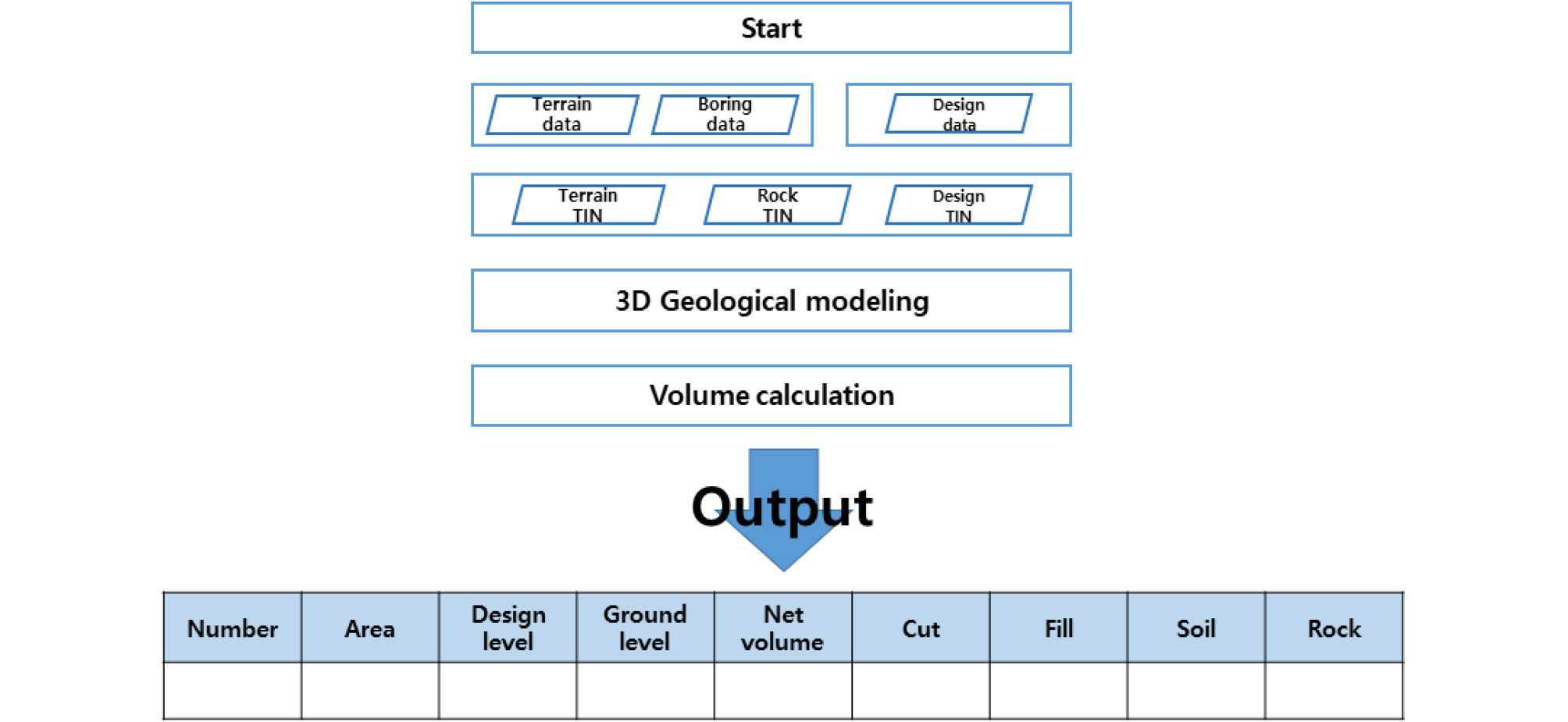
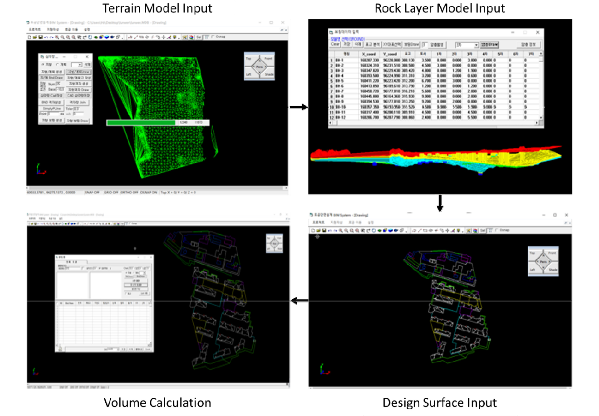
E-BIM is a tool for civil engineering design. The main functions are Drawing with point data. Using the boring data to make a rock formation model. Calculate volume of earthwork and rock. This system is based on V-Draw and CAD component using Visual basic 6.0. The flowchart of the system is shown in Figure 1 [20].
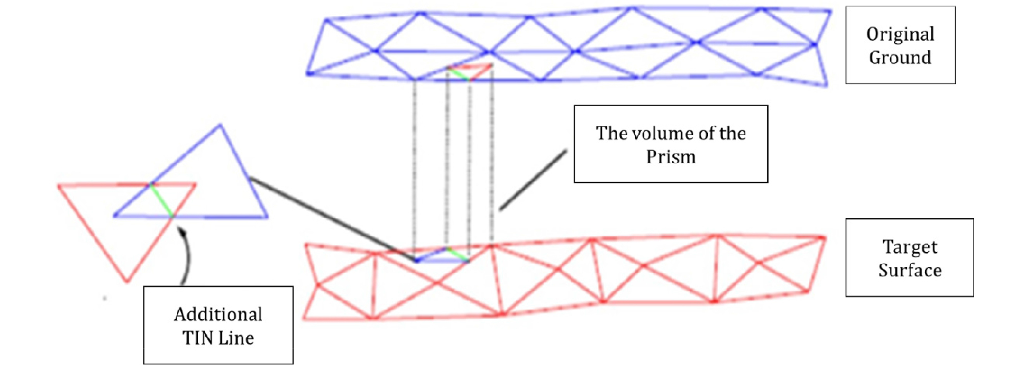
The most important factor to determine the precise design and technological plan of earthwork is the correct quantity of earthwork. Because of the amount of soil in the soil, the cost difference is extreme. The traditional method of volume calculation is to use topographic data and borehole data to create cross sections. Then the average and Ares methods are used to calculate the approximate number. Because of the characteristics of average and Ares methods, the longer the interval between cross sections or the greater the change of terrain, the more errors will occur. In addition, in the case of cross-section creation, because the cross-section can be different from the worker, the same data can be used to calculate different earthwork. The most representative method for calculating three-dimensional quantities is surface-to-surface method. When there are two surfaces in the three-dimensional volume calculation method, the face-to-face method is used. Triangulate on a new surface based on points on the old surface. The method creates a footnote segment in the composite triangle mesh using the intersection of the triangle mesh vertices between the two surfaces and the points on the two surfaces, and calculates a new composite surface elevation based on the difference between the elevations of the two surfaces. The process of calculating the quantity using the surface-to-surface method is as shown in Figure 2.
First, enter the Terrain TIN surface, Rock TIN surface, and Design data. Second, convert the design data to a TIN surface. Third, project a Terrain TIN surface and a Rock TIN surface onto the Design TIN surface. Fourth, calculate the centroid coordinate (x, y, z) of each projected TIN. Fifth, calculate the volume of triangular prism composed of existing TIN and projected TIN. Sixth, determine the Cut & Fill volume by comparing the z value of the center of the existing TIN with the z value of the projected TIN.
Case Study
Case introduction
The apartment construction project information as follow:
-Project Name: Jeju happiness, public rental apartment
-Project Location: Wolpyeong-dong apartment in Jeju island
-Project date:April 1st, 2018 – August 31st, 2018 (earthwork)
-Project detail: This is a foundation pit project with an area of 48,792m2, with a total of 23 areas. The average excavation depth is 5 m. There are 40 measured surface exploration data. The location and data of boreholes are shown in Figure 3 and Table 1.
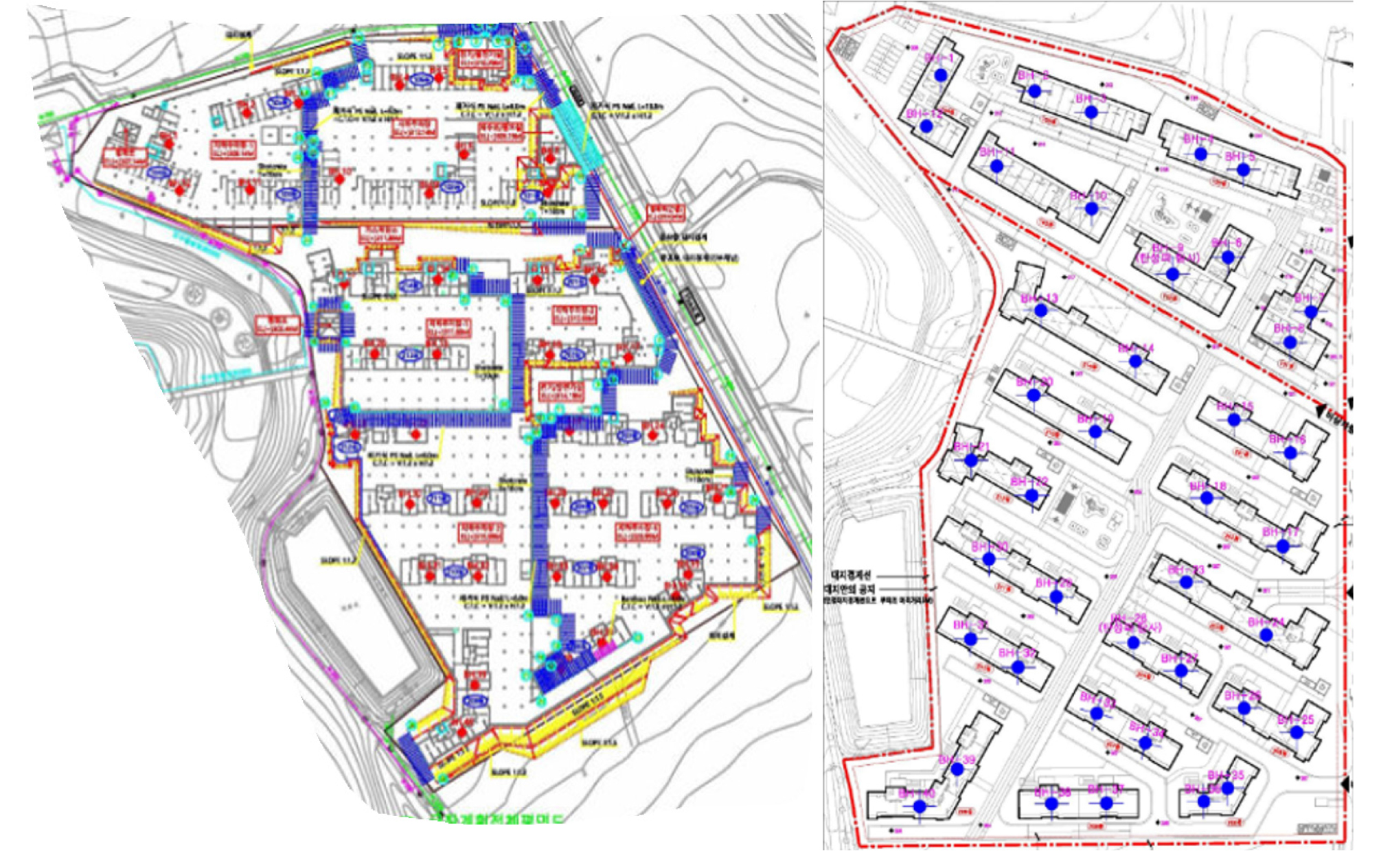
Table 1.
The location and data of boreholes
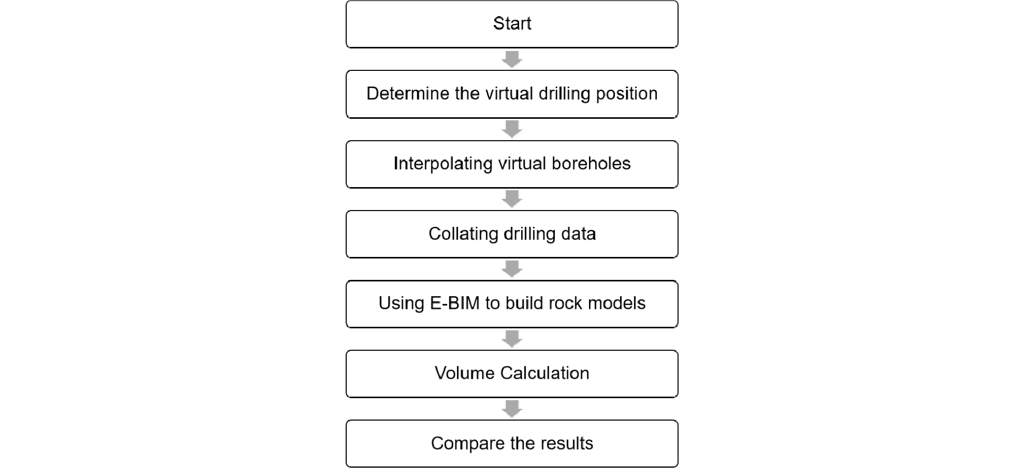
Generally, borehole data acquisition is obtained by engineers through various advanced scientific and technological means. Then it is integrated into tabular form, in which all rock data are mixed, so the boring data should be sorted out first. Then the location of the borehole is analyzed, virtual borehole is added, and the height of the virtual borehole is obtained by Kriging interpolation engineering, and the data is integrated, then the data is modeled and calculated by E-BIM. Finally, the results are compared as shown in Figure 4.
Result and Discussions
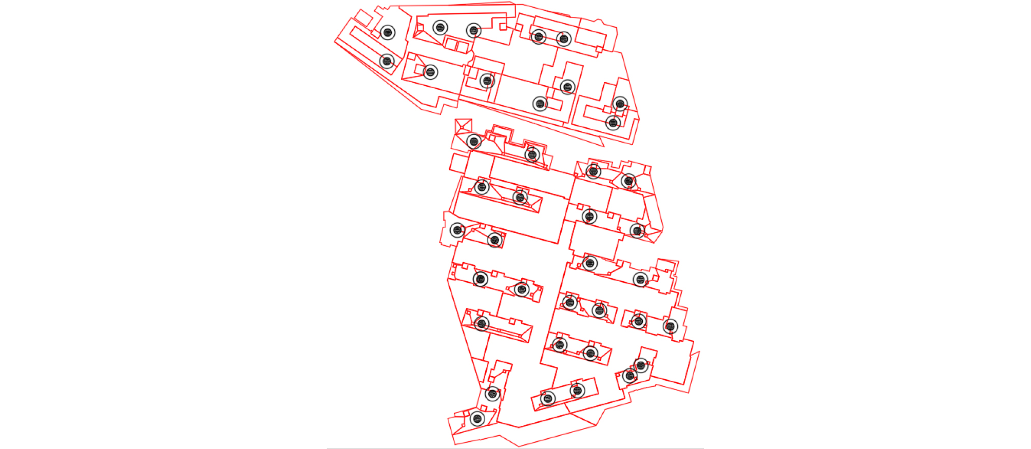
Through the analysis of the actual borehole distribution map of the project, the location of the virtual borehole is determined. The actual boreholes in the project are shown in Figure 5.
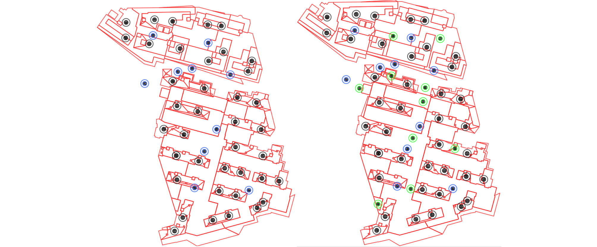
Through the analysis of location information, the virtual boring is established in the areas where boring data are evacuated. Two additions were made, each adding 10 virtual boring points. The location of the virtual boring hole is shown in the Figure 6.
After determining the virtual position through the previous step, the Kriging interpolation is used to interpolate the data of each stratum. The results of calculation are shown in Table 2 and 3.
Table 2.
1st add virtual boring
Table 3.
2nd add virtual boring
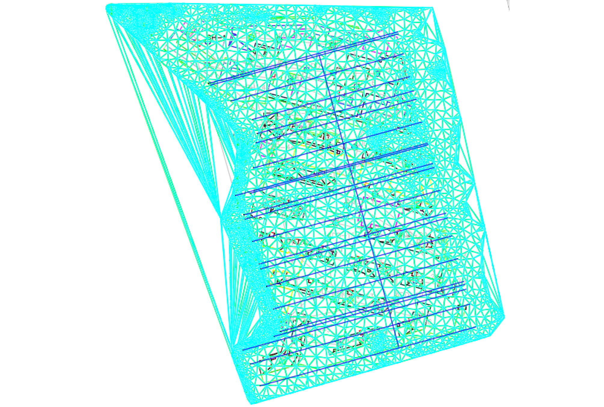
After the results are obtained, the data are sorted out. The interpolation results of each layer are integrated to form three layers of rock data for each borehole data. The following preparations should be made in advance for the use of E-BIM tools. Firstly, the original topographic map is imported into E-BIM, then the boring data integrated in the previous process is imported into E-BIM, and the design topography is created. The three-dimensional modeling is carried out by using the E- BIM modeling tool, and finally the quantitative calculation is carried out. Finally, the results are derived. The process (Figure 7) is as follows:
Using the original data, the volume of each rock layer is Rock 1 101.6 cubic meters, Rock 2 2408.49 cubic meters and Rock 3 3267.93 cubic meters. The total rock mass is 5793.8 cubic meters. After adding virtual boring data for the first time, the volume of each rock layer is Rock 185 cubic meters, Rock 2 is 2389.57 cubic meters and Rock 3 is 3568.48 cubic meters. The total rock mass is 6066.41 cubic meters. After adding virtual boring data for the second time, the volume of each rock layer is 71 cubic meters for Rock 1, 2456 cubic meters for Rock 2 and 3881.9 cubic meters for Rock 3. The total rock mass is 6285.6 cubic meters. The results table are shown in Table 4.
Table 4.
The result of the original boring (Unit: m3)
| Area | Rock 1 | Rock 2 | Rock 3 | Total |
| Original Boring | 101.6 | 2408.49 | 3567.93 | 5793.8 |
| 1st add virtual boring | 85 | 2389.57 | 3568.48 | 6066.41 |
| 2nd add virtual boring | 71 | 2456 | 3881.9 | 6285.6 |
| Actual | 65 | 2526 | 3960 | 6551 |
Because only the numerical results cannot be intuitive, clearly showing the difference between before and after interpolation, so I will build the model for cross-section processing. The cross-section diagram can better show the difference between the two. The position of the section line is shown in Figure 8 and 9.
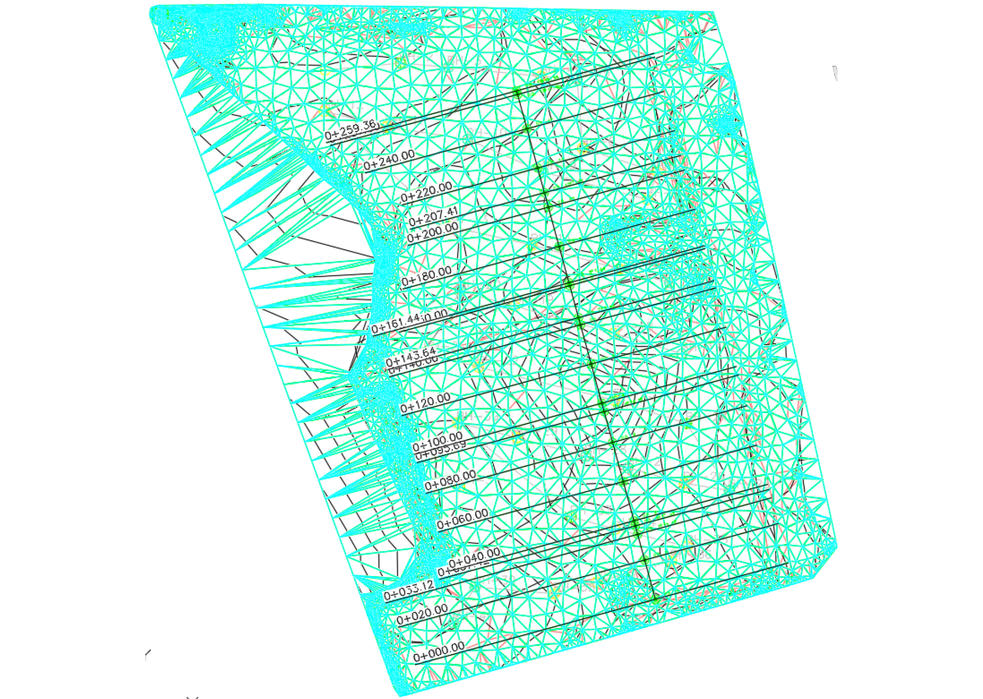
By comparing the cross-sectional maps, we can see the differences between the two before. Here are some details of the cross-sectional comparison. Because the difference between the 3 STA is obvious. Therefore, we chose these 3 stations as the demonstration. They are STA.0+20, STA.0+33.12, STA.0+37.42 as shown in Figure 10.
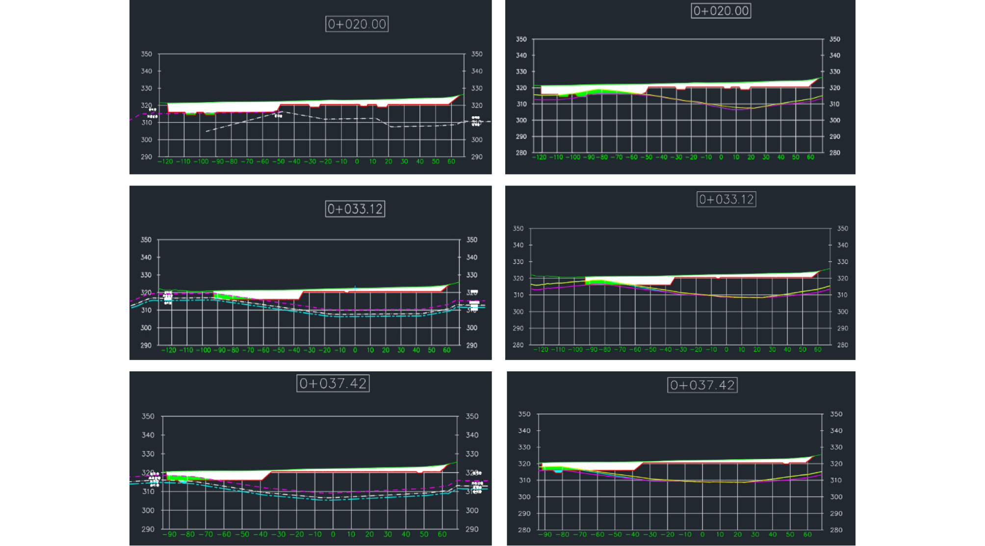
In the figure above, the original data is unused Kriging interpolation on the left and Kriging interpolation on the right. Different colors represent different rock types. In the contrast chart, we can clearly see the difference between the two. According to the actual data, the model after Kriging interpolation is more accurate than the original model. After volume calculation, the following results are obtained by error calculation. As a result, we can see that compared with the original data, the error after two interpolations is decreasing. This also shows that the data after Kriging interpolation is more accurate than the original data (Table 5). This implies that the Kriging interpolation can predict rock layers more accurately so that a construction manager may have more confidence of his/her equipment deployment decision
Conclusions
Spatial interpolation is the key technology of reconstructing geological environment, and it has been the focus of scholars all over the world. In this paper, the application of Kriging interpolation algorithm in three-dimensional geological spatial modeling is studied by using borehole data in the study area. From data preparation analysis, three-dimensional spatial variogram method and three-dimensional Kriging interpolation research to the final result of interpolation, the three-dimensional spatial geological attribute model is established. The spatial structure and anisotropic characteristics of geological environment are taken into account in the interpolation process. In the three-dimensional space, the Kriging interpolation of borehole data is used to build a three-dimensional geological model for analysis and research. The full text is summarized as follows:
The actual boring combined with the virtual boring of the Kriging interpolation makes the 3D model of the underground rock more intuitive and accurate.
In terms of scheduling, after obtaining a precise 3D model of the underground rock formation, the project can be more rationally planned. Shorten the construction period and further reduce total carbon emission.
In terms of cost, after a precise calculation, the budget error can be reduced.
