

Introduction
Literature Review
Demand Forecasting for Conventional Transportation
Traffic Demand Forecasting Using Deep Learning
Hybrid Transportation Demand Forecasting
Methodology
Gated Recurrent Unit
Genetic Algorithms
Hybrid Forecasting Model
Experiments
Results
Rental Forecasts
Return Forecasts
Discussion and Conclusions
Discussion
Conclusions
Introduction
Recently, mobility as a service (MaaS), which recognizes traveling as a service, has been in the spotlight. As new technologies are being applied to transportation, efficient use of the means of transportation, the optimization of transport networks, improved infrastructure utilization, and the development of business concepts for smooth traveling are being promoted. One of the business concepts in that process is MaaS, a service that combines public transportation, shared transportation (shared bikes, electric scooters, etc.), and taxis to promote convenient transportation [1]. It integrates various means of transportation, payment systems, and platforms into one service that is provided in an integrated way whenever needed [2]. To establish MaaS, the combination of new and traditional means of transportation is essential, and integrated data management and platform establishment are required [3, 4].
The purpose of MaaS is to integrate various means of transportation (public transportation, taxis, car sharing, public bikes, etc.) and services into a single user interface to provide seamless traveling and complete door-to-door service [5, 6, 7]. The best current examples of MaaS include Whim in Finland and UBiGo in Sweden.
Unlike traveling using existing public transportation, MaaS analyzes the entire process of traveling by taking service users as the scope of analysis, which emphasizes the importance of the first mile and last mile of travel [8]. To provide door-to-door services to customers, which is the purpose of MaaS, transportation services that can solve the first-last mile problem are required [9]. Micro mobility, such as public or shared bikes and scooters, is primarily used for short distances to facilitate connections between other means of transportation, particularly in the first-last mile of travel, thereby enabling seamless traveling. Micro mobility is thus an important component in maintaining the sustainability and efficiency of MaaS because it can solve the first-last mile problem and play a key role in facilitating the development of MaaS [9].
Currently, use information for micro mobility, including the locations of departures and arrivals, time of use, and distance of use, is tracked in real time and is accumulating. With the increase in demand for micro mobility, a vast amount of demand data is accumulating in real time, but it is not being processed into significant information [10]. Moreover, most micro mobility services manage demand only through real-time tracking, and thus preemptive responses to demand are inadequate [11]. Monitoring demand in real time alone is insufficient to respond to imbalances between supply and demand and cannot guarantee sufficient service quality [12].
To fully implement door-to-door services, which is the purpose of MaaS, and facilitate the convenience of service users, the integration of micro mobility to solve the first-last mile problem and the inclusion of demand forecasting to preemptively respond to demand are essential [13]. The development of MaaS requires the design and application of a demand forecasting model for micro mobility that can respond well to fluctuations.
This study was conducted to design and validate a demand forecasting model that can produce accurate forecasts in a short time by using micro mobility demand data that accumulate in real time and to introduce that model into MaaS to provide complete door-to-door services to users.
First, a real-time, deep learning–based demand forecasting model was designed by combining a genetic algorithm (GA), long short-term memory (LSTM), and gated recurrent unit (GRU) models. The LSTM and GRU, which are capable of time series analyses, are used as the forecasting models, and the GA is used to optimize the hyperparameters affecting their accuracy.
Second, micro mobility demand forecasting was performed using deep learning networks, and combined demand forecasting models (GA-LSTM, GA-GRU) were designed. Ttareungyi, the Seoul shared bike system and a representative example of micro mobility, was selected as the subject of study, and the forecasting models were applied to the station with the highest eigenvector centrality.
Third, the newly designed forecasting models were compared with RNN, LSTM, and GRU to validate the accuracy of the hybrid GA-LSTM and GA-GRU models.
Fourth, measures for MaaS development through micro mobility demand forecasting are presented, including the value that the combined demand forecasting models have for MaaS.
Literature Review
Demand Forecasting for Conventional Transportation
Demand forecasting in the transportation sector is generally carried out in pairs of origins and destinations, specifically forecasting cargo traffic volume, vehicle traffic volume, and the number of passengers departing and arriving. In particular, demand forecasting for transportation that is not privately owned, such as public transportation, rental cars, car sharing, and micro mobility, is the basis for the allocation/assignment of transportation and customer satisfaction because it manages the balance between supply and demand and profit maximization [14].
The time series forecasting models that have been conventionally used to forecast demand for public transportation by unspecified individuals (rather than privately owned vehicles) include analysis models such as moving average and exponential smoothing models, auto regressive moving average, autoregressive integrated moving average (ARIMA), which is also known as the Box-Jenkins model, and the Holt-Winters model [15, 16, 17].
Lim and Jeong [15] recognized the need for a robust demand forecasting method to predict the daily number of shared bikes rented in Seoul and used the Holt-Winters model. They concluded that the rental predictions could be used to relocate shared bikes. However, they presented the need to forecast rentals using more data to appropriately reflect seasonality and suggested comparing the forecasting performance of ARIMA with those of machine learning methods as a future research direction. Lee and Kwon [18] established a dynamic change model for transportation demand using the SARIMA (seasonal ARIMA) model and railway traffic performance data. They noted that SARIMA has the advantage of eliminating the need for information about explanatory variables in future forecasts, but it has difficulty reflecting planned structural changes for the future. Kumar and Vanajakshi [19] applied SARIMA to forecast short-term traffic flows. They noted that several previous studies had shown the SARIMA model to have better forecasting performance than linear regression, support vector regression (SVR), and the basic ARIMA model. The implication of the study of Kumar and Vanajakshi [19] is that their SARIMA results are accurate enough to be applied to an intelligent transportation system. Danfeng and Jing [20] forecast the number of subway passengers in Guangzhou using ARIMA, GBRT, a deep neural network (DNN), LSTM, and DA-RNN models. They stressed that forecasting the number of passengers accurately is a critical part of establishing smart city services. They tallied up passenger flows every 10 minutes, forecast the number of passengers arriving and departing at the station using 5 models, and compared the accuracy of the models. They found that the ARIMA model had disadvantages of not being able to derive nonlinear relationships between widely used models or variables when forecasting the number subway passengers and of showing a decline in accuracy during long-term forecasting. Among the five models they tested, the ARIMA model had the lowest forecasting performance.
Forecasting models are still being developed, and forecasts are being performed in a variety of ways using time series analysis models such as ARIMA, but the conventional statistical-based time series analysis models have clear disadvantages, such as fundamentally forecasting linear demand and requiring assumptions that make it difficult to forecast fluctuating demand changes in the real world [16]. The forecasting methods used to predict short-term traffic demand can be divided largely into parametric approaches, represented by ARIMA, and non-parametric approaches, represented by LSTM and GRU. Parametric approaches have the advantages of being simple and easy to understand, and they can make good forecasts when fluctuations in traffic demand are small, but irregular fluctuations in demand produce large forecast errors [21, 22]. Demand forecasting for means of transportation with high demand volatility, such as micro mobility, is difficult to do using parametric and statistical methods because it requires models that can predict nonlinear demand.
Traffic Demand Forecasting Using Deep Learning
The main advantage of deep learning is that nonlinear modeling is possible [16]. Recently, researchers have begun using artificial neural networks and evolution algorithms rather than conventional statistical forecasting methods such as ARIMA for forecasting [23]. Short-term traffic demand forecasting based on data-driven methods such as artificial neural networks is an actively evolving field of research [23].
The emergence of new means of transportation for the first and last mile and new transportation services, such as MaaS, is producing a massive amount of information on traffic demand that is being collected and accumulated in real time. Some published studies have shown that when demand is changing in real-time and data are being collected—that is, when nonlinear demand occurs and is recorded—demand forecasting methods that use deep learning algorithms are more accurate than earlier forecasting models that use conventional statistical methods and parametric approaches to forecast demand [12, 21, 22, 24].
Fu et al. [22] determined that because traffic demand has nonlinear characteristics, forecasting using deep learning models is more suitable than time series models, and they found that recurrent neural networks such as LSTM and GRU have smaller forecasting errors than ARIMA in forecasting short-term traffic demand, with GRU outperforming LSTM. Ruffieux [12] used a random forest, a machine learning technique, and a convolutional neural network (CNN) to forecast the real-time use of bike sharing systems. He found that the random forest algorithm had better forecasting accuracy for relatively short (5 minutes) times whereas the CNN had better forecasting accuracy for relatively long (60 minutes) times. Zhao et al. [21] used the LSTM model for short-term traffic demand forecasting in Beijing and compared the forecasts for 15, 30, 45, and 60 minutes made using the ARIMA, SVM, RBF, SAE, and RNN models. They showed that the forecasting performance of models using LSTM was better than that of the other forecasting models. Pan et al. [25] applied LSTM in their real-time method to predict the number of rented and returned bikes. Kim et al. [26] compared the forecasting performance of ARIMA, a neural network, an Elman recurrent neural network model, and LSTM by applying all of them to data on the number of passengers on international airlines. They found that the Elman recurrent neural network model showed the best forecasting performance, and the LSTM model showed superior fitness to the ARIMA model and Faraway’s basic neural network model. Cho et al. [24] developed a LSTM-based deep learning model to predict public bike rentals and suggested that using the LSTM forecasting method to predict public bike rentals could significantly reduce forecast errors compared with the exponential smoothing model and ARIMA.
Forecasting models that use deep learning algorithms are needed to address complex demand patterns in the real world and advance forecasting models, and studies showing that they have high forecasting accuracy are being published. However, a disadvantage of using deep learning algorithms for demand forecasting is that their accuracy varies significantly according to the hyperparameters, which have a major influence on deep learning [27]. Demand forecasting methods such as LSTM and GRU, which are used in deep learning, especially in time series analyses, are better than statistical time series forecasting methods for forecasting nonlinear demand, but the hyperparameters required for training, such as epoch and batch size, directly affect their forecasting performance and must be subjectively determined. The forecasting process must then be repeated to find suitable hyperparameters, resulting in substantial computational costs [27, 28].
Hybrid Transportation Demand Forecasting
Studies about the optimization of the hyperparameters used in machine learning and deep learning are also being published. Hyperparameters are not values determined by machine learning; they are established prior to the learning process and directly affect the accuracy of the models [28]. In other words, deep learning techniques require that hyperparameters such as epoch, the number of neurons, the learning rate, and batch size be established prior to data training. Moreover, optimal hyperparameters can improve the accuracy of the resulting forecasting models, so optimization—finding the best hyperparameters—requires trial and error processes by researchers and hands-on workers to maximize the accuracy of the forecasting models. A hybrid forecasting model that can use algorithms for hyperparameter optimization to speed the production of deep learning models is being developed in this work. Various exploration measures are being proposed to achieve the optimal hyperparameters, including random search, grid search, and Bayesian optimization. Methods that combine metaheuristic algorithms, including GAs, differential evolution, particle swarm optimization, simulated annealing (SA), and TABU searches, are being studied as well.
Bui and Yi [29] revealed that deep learning algorithms (SAE, LSTM, CNN, etc.) can show a high degree of accuracy in forecasting demand by using large amounts of traffic data, but determining their hyperparameters is difficult. Before forecasting demand using LSTM, they used the Bayesian optimization method to determine the hyperparameters, which are the batch size, learning rate, number of neurons, and drop-outs. Tsai et al. [30] used SA to determine the number of neurons, one of the deep learning hyperparameters, to forecast the number of bus passengers. They confirmed that better forecasting performance was shown when applying the number of neurons derived by SA to DNN rather than when forecasting the number of bus passengers using a support vector machine, random forest, or DNN single model. Li et al. [31] combined evolutionary attention (EA) with LSTM to determine the number of layers and compared its forecasting performance with that of SVR, GBRT, RNN, GRU, LSTM, Attention-LSTM, and DA-RNN models. The results from measuring the accuracy of the forecasting models using the root mean square error (RMSE) and mean absolute error (MAE) showed that the EA-LSTM achieved the best forecasting performance. Tang et al. [32] used a GA to produce the hyperparameters (batch size, epoch, and hidden units in each layer) for LSTM and tested the forecasting accuracy of their GA-LSTM model against six other models. Their GA-LSTM model produced the best forecasting performance.
In most studies, only the number of neurons in the hidden state, batch size, etc., are tested to improve the forecasting accuracy of artificial neural network models; however, numerous hyperparameters must be considered simultaneously to optimize the accuracy of forecasting models. This study simultaneously optimizes the window size, number of neurons in the hidden state, epoch, learning rate, and batch size to improve forecasting accuracy and then applies those values to artificial neural networks to perform demand forecasting.
Methodology
Gated Recurrent Unit
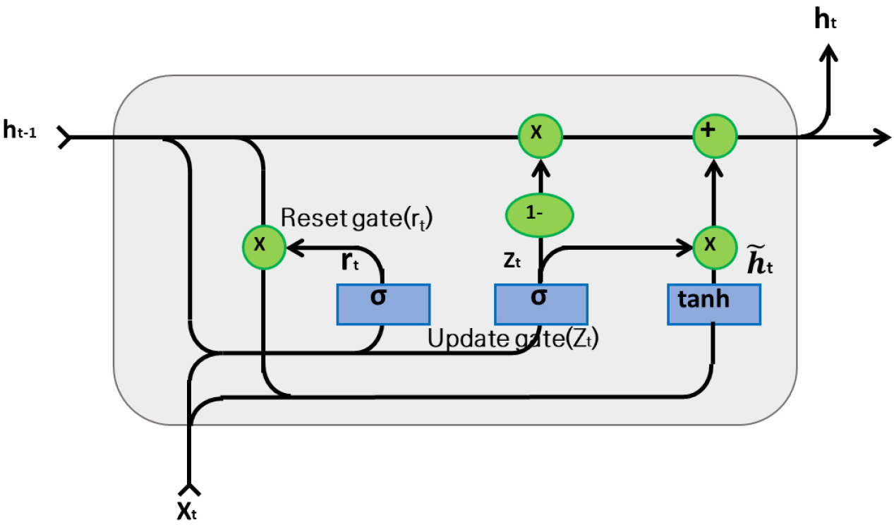
The GRU is a deformation model that simplifies the structure of LSTM [33, 34]. Like LSTM, it was developed to address an RNN’s vanishing gradient and short- and long-term dependence on an exploding gradient. The GRU, due to its cell structure, can perform calculations more quickly than LSTM without significant differences in performance [33]. Whereas LSTM is made up of three gates, GRU is composed of two gates, the reset gate and the update gate.
In the hidden layer in the GRU model, the reset gate initializes past information, and the update gate determines the update rate for past and present data. The reset gate determines how much value from the previous hidden state to use.
In other words, the role of the reset gate is to erase past information, whereas the update gate has functions similar to those of both the input gate and forget gate in LSTM, which determine how much data from the previous step and the current step are reflected, respectively.
In Figure 1, zt is the update gate, and rt is the reset gate. t is an internal hidden node candidate value, ht is the final hidden node output value, and 𝑥t is the input value at time t. 𝑊z, 𝑊r, and 𝑊c are weight matrices connected to the input vector 𝑥t. z, r, and c are weight matrices connected to the short-term state ht-1, and bz and br denote bias. A GRU can be trained with a relatively small amount of data because it has a smaller number of weights and biases than LSTM, but LSTM can achieve better forecasting results when more data are available.
In addition, LSTM and GRU can handle longer sequences than a simple RNN, but they have limited short-term memory, and they sometimes have difficulty learning long-term patterns in sequences of 100 time steps or above. To compensate for that, a method of shortening input sequences using 1D convolution layers is used [35]. In this study, a GRU is used as a hybrid forecasting model in combination with a single forecasting model and GAs, just as with LSTM.
Genetic Algorithms
GAs form the backbone of a variety of evolutionary algorithms and are the most widely applied algorithms. They are metaheuristic and stochastic optimization algorithms based on the natural evolution process [36, 37, 38]. One characteristic of GAs is their ability to find a global optimum solution or an optimum solution that is almost the same as the global optimum solution in a limited time using a population that contains multiple potential solutions [39].
In GAs, chromosomes represent arbitrary solutions, and groups of chromosomes are called populations. The factors that make up chromosomes are called genes, and a gene is the smallest unit of a GA. In this study, real numbers were used for chromosome expression, and five genes were set to compose each chromosome, which are the hyperparameters of the LSTM and GRU.
A GA runs the processes of repeated selection, crossover, and mutation based on probability to find solutions that minimize or maximize fitness functions. Genetic algorithms are conducted using the following procedures: formation of the initial population, fitness function evaluation, selection, crossover, mutation, fitness function evaluation, and exit criteria verification.
The first phase in a GA is the formation of the initial population. Heuristic or arbitrary methods are used to generate the initial population. In the second step, fitness is evaluated according to the purpose of the optimization and can be evaluated using the minimum value, maximum value, etc. for that purpose. The third step, selection, selects which individuals will survive in the next generation based on the fitness of the chromosomes. The selection methods include tournament selection, roulette wheel, and ranking selection. The tournament selection method was used in this study. The fourth step is crossover, in which new chromosomes are created from the chromosomes that survived the selection stage, that is, the solutions. In this study, a two-point crossover method was used. The fifth step, mutation, transforms some of the genes on the chromosomes with a specific probability to explore the solution space in a variety of ways, contributing to group diversity. In the sixth step, fitness evaluation, the fitness of the chromosomes generated through the preceding five steps is evaluated. The whole process ends when the exit criteria designated as the hyperparameters are met in the final step of exit criteria verification. If the exit criteria are not met, the process returns to the selection step and repeats from there as needed.
Hybrid Forecasting Model
Finding suitable hyperparameters is a major issue in machine learning. Deep learning algorithms such as LSTM and GRU change their parameters through a learning process that uses the input data. On the other hand, although the hyperparameters used in deep learning have a significant effect on the performance of the resulting models, they do not change with the learning process and must be set before training. When developing forecasting models that use deep learning, the challenge is to find the optimal hyperparameter values through an iterative trial and error process. Models based on artificial neural networks, such as RNN, LSTM, and GRU, have numerous hyperparameters that greatly affect their forecasting performance. It is difficult to find suitable hyperparameter values if the decision maker has little experience in the corresponding field [27]. Numerous studies of deep learning networks have used change processes to search for suitable hyperparameters. The computational cost of hyperparameter optimization is extremely high because it requires an iterative calculation process.
Finding optimal hyperparameters is a NP-hard (nondeterministic polynomial-hard) question. GAs are known to be an effective model for solving NP problems in diverse fields [39]. In this study, GAs are used for hyperparameter optimization of deep learning models to minimize the loss function. Among the many hyperparameters, five were chosen: window size, number of neurons in the hidden state, batch size, epoch, and learning rate.
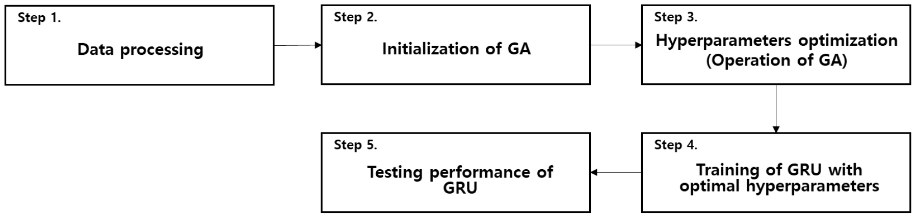
After the GAs set up those five hyperparameters for the LSTM and GRU, they were applied to forecast demand with high accuracy. To achieve forecasts by combining GAs with LSTM and GRU, a five-step forecasting process was used. Figure 2 illustrates the procedures for making forecasts by combining GAs and GRU.
Experiments
The purpose of this study is to improve the accuracy of forecasts for micro mobility demand to advance MaaS. To realize that object, models that can make accurate forecasts in a short time are designed to use demand data that accumulate in real time. This paper forecasts the rentals and returns of a micro mobility system over time.
The subject of this study was Seoul City’s public bike service, Ttareungyi. The time, place, etc., of Ttareungyi rentals and returns are tracked in real time, and the accumulated data can be extracted through Seoul Open Data Plaza (http://data.seoul.go.kr), including daily and monthly data.
In this study, ‘Seoul Metropolitan City Public Bike Rental History Information’ data from January 1, 2019, to December 31, 2019, were collected from Seoul Open Data Plaza and used. The ‘Seoul Metropolitan City Public Bike Rental History Information’ data contain the number of bikes, date and time of rental, number and name of rental stations, rental stands, date and time of return, number of rental station for return, return stand, time of use (unit: minutes), and distance of use (unit: m). For the usage behavior analysis and demand forecasting, outliers, such as a recorded time or distance of zero, were removed. Among the total 1553 Ttareungyi stations, the station with the highest centrality is station 2219 (Station name: Express Bus Terminal Station; between exit 8-1 and exit 8-2). The rentals and returns were forecast using the rental data for that station from January 1, 2019, to December 31, 2019, and applying the hybrid models developed here (GA-LSTM, GA-GRU).
Hourly rentals and returns were aggregated and applied to the forecasting models by using the relevant basic data. To measure the accuracy of the GA-GRU model, its forecast was first compared with the actual Ttareungyi rentals and returns, and it was then compared with predictions from other models (RNN, LSTM, and GRU).
Before performing the forecast, the Ttareungyi rental and return data were processed. The data were normalized using the min-max normalization method to eliminate noise and improve forecasting accuracy.
is the source data (hourly number of Ttareungyi rented and returned), and max and min are the maximum and minimum values in the data set of rentals and returns. is a normalized value between 0 and 1.
To perform the training, adaptive moment estimation (Adam) was applied as the optimizer. Adam is a technique for efficient optimization and is studied based on the AdaGrad method. Adam reflects some past information in the update by momentum and derives the final update size in combination with the newly calculated gradient direction.
To verify the demand forecasting model, computers installed with Intel i7-9700 3.0GHz, 64GB RAM, and NVIDIA Geforce RTX 2060 SUPER graphic cards were used. The development environment used Tensorflow2.0 and Python 3.6, and the Distributed Evolutionary Algorithm in Python calculation framework was used to apply the GAs.
To achieve optimal hyperparameters, the range of hyperparameters that the GAs could explore needed to be set. Table 1 provides the range of hyperparameters established in this study.
Table 1.
Range of Hyperparameters
| Hyperparameter | Range |
| Window size | [1, 30] |
| Number of neurons in the hidden state | [1, 50] |
| Batch size | [1, 50] |
| Epoch size | [10, 300] |
| Initial learning rate | [0.0001, 0.001] |
When the single time series forecasting models (RNN, LSTM, and GRU) were learning the data and deriving forecasts, the average values from the ranges specified in Table 1 were used for the hyperparameters.
The GA parameters, population size, number of generations, crossover probability, and mutation factors, were set based on previous studies. Optimal parameters are not designated, but such decisions are made by analyzing each application problem [36]. GAs do not produce good results with a small population size or small number of generations. The population size and number of generations should be at least five [40]. Table 2 demonstrates the range of parameters established in this study.
Table 2.
Range of Parameters
| Parameter | Range |
| Population size | 10 |
| Number of generations | 15 |
| Crossover probability | 0.65 |
| Mutation factor | 0.015 |
In this study, the population size was set to 10, and the number of generations was set to 15. Moreover, the crossover probability and mutation factors are generally set between 0.5 and 1.0 and between 0.005 and 0.05, respectively [41]. In this study, the crossover probability for the GA was set at 0.65, and the mutation factor was set at 0.015.
The accuracy of the demand forecasting models was measured using MAE and RMSE, which are calculated as follows. N is the number of time series forecasting input data, yi is the real value, and fi is the predicted value.
Station-level demand forecasting by time is the basis for expanding the system design for transportation services and helps to maintain an appropriate number of bikes [42]. In this study, a network analysis focused on the connection between stations based on the annual rentals and returns of Seoul City’s Ttareungyi in 2019. Considering the future arrangement of Ttareungyi, the station that can be the hub, or the station with the highest eigenvector centrality, was selected as the representative station. The hybrid forecasting model was applied to that station to forecast the number of bikes rented and returned, and the accuracy of the forecast demand was measured using MAE and RMSE.
Results
Rental Forecasts
The number of bikes rented at station 2219 in 2019 was 64,265, with an average time and distance of use of about 51 minutes and 7,311 meters, respectively. As a result of reclassifying the data on a 51-minute basis, the time scale was aggregated at 10,305 cases. The horizontal axis of the graph is the unit of time recorded for one year every 51 minutes, and the vertical axis is the number of bikes rented in each time unit. In 2019, the standard deviation of rentals was 9.55, with a minimum demand of 0 bikes, a maximum demand of 78 bikes and an average demand of 6.24 bikes every 51 minutes.
The 64,265 rental data at station 2219 were thus reclassified based on the rentals (demand) that occurred every 51 minutes (the average time of use), and the data set used for the validation of the final forecasting model was 10,305 cases. Of those, 7,214 observed values were used as the training set (70%), 1,030 were used as the validation set (10%), and 2,061 were used as the test set (20%).
The comparison of the single-method demand forecasting models (RNN, LSTM, and GRU) with the GA-LSTM and GA-GRU hybrid models is shown in Table 3.
Table 3.
Accuracy of the Rental Forecasting Models
The results of the accuracy comparisons show that the GA-GRU model had the highest accuracy when the percent deviation of each model was calculated based on the RNN. The forecasting accuracy difference in the models was calculated as 100×(R-Rfm)/R, where R is the RMSE and MAE of the RNN, and Rfm is the RMSE and MAE of the other forecasting models (RNN, LSTM, GRU, GA-LSTM, GA-GRU). The forecasting accuracy of the models approached the actual demand in the following order (from best to worst): GA-GRU, GA-LSTM, LSTM, GRU, and RNN. The GA-GRU model showed 12.23% better forecasting accuracy than the RNN model based on RMSE and 12.16% better forecasting accuracy based on MAE.
Return Forecasts
In the Ttareungyi data used to forecast the number of bikes returned, 51 minutes, which was the criterion for aggregating the number of bikes rented at station 2219 (Station name: Express Bus Terminal Station; between exit 8-1 and exit 8-2), was also set as the standard time for aggregating the number of returned bikes. In 2019, 68,115 Ttareungyi were returned to station number 2219.
When the return data were reclassified and aggregated based on the average time of use of 51 minutes, the return status of Ttareungyi at station number 2219 in 2019 had a minimum of 0 bikes, maximum of 93 bikes, and average of 6.6 bikes per 51 minutes, with a standard deviation of 10.38.
After reclassifying the data by dividing the time into 51-minute intervals, the time axis was classified into 10,305 units, which is the same as the number of time units for the number of rented bikes at station number 2219, indicating that no bikes rented on December 31, 2019, were returned in the next year on January 1, 2020.
The data used for training, validation, and testing of the hybrid forecasting models were separated into 10,305 units, with 7,213 used as the training set (70%), 1,030 used as the validation set (10%), and 2,061 used as the test set (20%).
The comparison of the single-method demand forecasting models (RNN, LSTM, and GRU) with the hybrid GA-LSTM and GA-GRU models is shown in Table 4. Table 4 compares the accuracy of the single recurrent neural network forecasting models and the recurrent neural network models combined with GAs. The model with the best forecasting performance was the GA-LSTM model, which had a return forecasting accuracy of 3.261 by RMSE and 1.987 by MAE.
Table 4.
Accuracy of Return Forecasting Models
The accuracy difference of the forecasting models was calculated as 100×(R-Rfm)/R, where R is the RMSE and MAE value of the RNN, and Rfm is the RMSE and MAE value of the other forecasting models (RNN, LSTM, GRU, GA-LSTM, GA-GRU). The GA-LSTM model showed 8.32% better forecasting accuracy than the RNN model based on RMSE and 11.73% better forecasting accuracy based on MAE.
Discussion and Conclusions
The hybrid forecasting model presented in this study exhibited better forecasting accuracy than the single forecasting models tested. Designing a demand forecasting model for micro mobility and increasing its forecasting accuracy is essential because providing MaaS customers with information based on predictions (rentals and returns) will allow them to make transportation decisions based on that information, which is directly related to customer satisfaction. Therefore, accurate forecasts must be derived and reflected in MaaS systems and platforms. Also, from the operators’ perspective, accurate rental and return forecasts that match times and places are required for efficient relocation of equipment.
Using the hybrid demand forecasting methods (GA-LSTM, GA-GRU) presented and validated in this study, MaaS operators can provide valuable information to users and promote efficient demand and supply management. Furthermore, MaaS operators can compare rental forecasts with real-time rental tracking to determine how many bikes should be procured or relocated at which times and to which stations. Return forecasts can provide MaaS users with information about the number of bikes expected to be at a station at a particular time based on the difference between the predicted rentals and predicted returns. If a deficiency in the supply is predicted at a certain time and place, demand and customer satisfaction can be managed through MaaS by providing guidance services for a different route where an adequate supply of bikes is forecast.
In this study, the number of bikes rented and returned was forecast based on the average time of use; however, when applying the hybrid forecasting model in practice, different time steps could be used by tracking and aggregating rentals and returns every 5 or 10 minutes. To provide information valuable to MaaS users, there is a need to determine the best unit of forecasting time.
To practically apply forecasts of rentals and returns for micro mobility units, future MaaS platform operators should be able to integrate hybrid forecasting models with parallel computing techniques such as Hadoop or Spark. Establishing such a system architecture will make it possible for hybrid demand forecasting based on real-time demand data to be applied practically so that users can open a MaaS application and receive advanced mobile information, such as the number of bikes expected at their station at their intended arrival time and route guidance services. In addition, it would allow operators (such as transportation companies) to determine the number of deployments needed, movement locations, etc.
Further research into the following topics is needed to compensate for the limitations of this study. First, it has been shown that GAs can be used to optimize hyperparameters and that doing so improves forecasting performance over that available from single deep learning techniques, but it is necessary to compare the forecasting performance available from combining other metaheuristic methods, such as SA and TABU searches, to see whether a better hyperparameter optimization method can be found.
Second, various micro mobility modalities can be incorporated into MaaS, such as dockless public bikes and electric scooters, and thus in the future, demand forecasting should be performed with expanded research subjects. In particular, for micro mobility systems such as shared bikes and electric scooters that are already operating without the need for stations or stands, the hybrid forecasting methods used in this study might not be suitable.
Third, to apply the demand forecasting methods suggested by this study to an actual MaaS system from a practical perspective, a concrete system architecture would need to be established. Furthermore, to determine the number of deployments needed at each station, an additional analysis of the proximity between stations must be performed to form batch clusters.
Conclusions
This study proposed GAs as a way to explore the hyperparameters of LSTM and GRU and designed and validated GA-LSTM and GA-GRU hybrid demand forecasting models.
This study has the following academic and practical implications. Academically, it is meaningful first in that it designed a forecasting model suitable for nonlinear demand forecasting and verified the accuracy of that model. Conventional time series forecasting methods in the transportation field have used parametric approaches such as ARIMA, which produce linear results. That’s a problem when the actual demand is highly variable and nonlinear. The demand forecasting method presented in this study, which combines GAs with LSTM and GRU, has been validated through previous studies and public bike data and shown to be advantageous in forecasting highly variable demand.
Second, this study contributes to the development of automated machine learning by performing hyperparameter optimization through algorithms rather than through subjective researcher activity. A disadvantage of deep learning networks is that optimizing the hyperparameters, which directly affect the forecasting performance of the model, is difficult. In many studies that use deep learning techniques, optimal hyperparameters are searched for, and repeated experiments are conducted to vary the hyperparameters and thereby improve the forecasting accuracy of the models. This results in huge computational costs, and searching for optimal hyperparameters remains challenging despite multiple experiments. In this study, hyperparameter optimization was performed by applying GAs
Practically, this study expanded the real-time demand predictability of micro mobility by applying the GA-LSTM and GA-GRU models to micro mobility demand forecasting. Among the means of transportation within MaaS, micro mobility focuses on the first-last mile range. Demand forecasting for micro mobility enables MaaS users to preemptively respond to changes in service availability. Preemptive responses and real-time tracking of the means of transportation require forecasting, and this study has presented a forecasting method that can be applied to MaaS by applying data that are already accumulating in real time to forecasting models.
Second, this study has provided a way to apply the forecasts derived from the hybrid forecasting model to MaaS, thereby enhancing its value and the satisfaction of service users and increasing the operational efficiency of MaaS suppliers. When a MaaS application forecasts the number of rentals and returns of micro mobility units and provides the expected number of bikes remaining, service users will be able to determine whether the means of transportation they wish to use will be available when they arrive, and suppliers will be able to determine when and where they need to deploy which means of transportation.
