

Introduction
Literature Review
Data and Methods
Study area
Data
Methods
Results
Prediction model
Descriptive statistics
How the urban built environment affects commuting distance
Nonlinear relationship between the urban built environment and commuting distance
Discussion and Conclusions
Introduction
Commuting is an essential part of urban life [1] and contributes to global environmental issues. The transportation sector is a significant source of greenhouse gas (GHG) emissions [2], and daily commuting accounts for a large portion of total trips and has a significant impact on emissions and congestion [3]. Consequently, analyses of individual commuting behaviors have been actively conducted with the goal of reducing commuting distances [4]. Additionally, the recent increase in long-distance commuting not only exacerbates existing environmental problems but is also linked to urban problems such as urban sprawl [5]. Thus, understanding the determinants of commuting distance from a planning perspective is crucial to identify suitable urban forms and built environments to reduce commuting distances and effectively manage them through spatial planning [6].
From a policy perspective, the built environment refers to artificially created surroundings for human activities [7], including urban design, land use, transportation systems, and human activity patterns [8]. Understanding the built environment’s impact on travel is valuable for developing measures to reduce energy consumption and transport emissions [9]. Moreover, assessing these impacts in advance is critical, considering the substantial time required for constructing urban built environments [10].
Nevertheless, existing studies have been mostly conducted in Western cities [7] with contradictory results on the relationship between certain built environment variables and commuting distances due to their use of traditional statistical methods that assume a linear relationship and failure to consider the evolution of the urban environment [11]. This highlights the need for a comprehensive analysis of the relationship between built environments and commuting distance in various urban contexts.
Recently, advancements in big data, such as mobile phone data, have enabled accurate predictions of various social phenomena and a better understanding of the nonlinear relationships among variables. Mobile phone data provide substantial amounts of real-time data at a lower cost [12], encompassing spatiotemporal information related to human movement [13]. They provide finer spatial detail than travel survey data, enabling more precise insights. Thus, they enables the capture of individuals’ movement patterns with high spatiotemporal resolution, underscoring their potential for predicting human movement behavior [14, 15]. Additionally, machine learning (ML) algorithms can learn from big data and construct models that can predict targets with high accuracy, they have been applied to predict diverse social phenomena [16, 17]. Furthermore, in addition to providing accurate predictions, the prediction process can be understood by applying explainable ML (XML) techniques by capturing the contribution of variables and nonlinear relationships observed during the prediction process [18].
In summary, predicting individual commuting distances using urban built environment data and analyzing variable impacts can effectively support spatial planning. Big data and ML techniques enable more accurate commuting distance predictions and facilitate the identification of nonlinear relationships between built environment factors and commuting distances during prediction.
This study aims to examine nonlinear relationship between urban built environment and commuting distance in Seoul using big data and XML techniques. The remainder of this paper is structured as follows. Section 2 reviews the literature on the relationship between built environments and commuting distance. Section 3 introduces our study area, data, and ML techniques, while Section 4 presents the analysis results. Section 5 discusses the results and summarizes the conclusions.
Literature Review
Analyzing the determinants of commuting patterns has long been a significant research topic [19]. Unlike trip frequency and mode choice, built environment variables have a greater impact on trip length than socioeconomic variables [20]. Cervero and Kockelman [21] proposed the D variables, including density, diversity, and design, as the primary characteristics of land use and built environment. Subsequently, new D variables, such as destination accessibility and public transportation accessibility, have been used.
Density, referring to the compactness of development, is typically assessed using population, residential, and employment densities. Higher residential density tends to reduce travel distances, including commuting distances [22, 23, 24]. This suggests that the high-density urban form resulting from compact development effectively reduces travel distance in Western cities. However, other findings suggest no significant relationship between population density (or residential density) and commuting distance in Asian cities [25, 26], potentially indicating that high-density urban form strategies may not effectively reduce commuting distances in Asian cities. Therefore, the relationship between density and commuting distance remains unclear, necessitating further empirical studies in diverse urban contexts.
From the perspective of diversity variables, mixed land use and job-housing balance can contribute to reducing commuting distances [27]. Specifically, there is a correlation between high density and mixed land use, and the latter tends to reduce commuting distances [9, 28, 29]. By utilizing job-housing balance as a diversity variable, Cervero and Duncan [30] found that a high level of job-housing balance reduces vehicle miles traveled (VMT). However, lower levels of job- housing balance increase long-distance commuting by public transportation and cross-commuting [31].
Destination accessibility refers to the distance to the urban employment center, commonly known as the central business district (CBD). The distance from residence to the CBD is identified as the most significant factor influencing commuting distance in numerous studies. The commuting distance increases when the residence is farther from the CBD [32, 33, 34]. Accordingly, unlike other variables, the distance to the CBD shows consistent results in many studies.
Meanwhile, regarding commuting mode, public transportation accessibility has an unclear relationship with commuting distance. Van Acker and Witlox [35] reported that as the distance from the residence to bus stops increases, the commuting distance tends to increase, suggesting that low public transportation accessibility in residential areas may lead to long- distance commuting. However, other studies have reported that commuting distance tends to increase with better accessibility to railways [36]. Additionally, Zhao [7] found that higher public transportation density in outskirt areas is associated with an increased likelihood of commuting to the city center. This finding suggests that both cars and public transportation are used as primary modes of long-distance commuting in some study areas due to congestion in the city center. Therefore, empirical evidence on the relationship between public transportation accessibility and commuting distance in various urban contexts is needed.
Existing studies report that the built environment at the residence significantly affects commuting distance, primarily focusing on the relationship between this environment, which serves as the origin of commuting, and commuting distance. Meanwhile, few studies analyze the relationship between the built environment at the workplace and commuting distance. These studies report that factors such as workplace density [23], distance from the workplace to the city center and CBD [32, 34, 36], and public transportation accessibility at the workplace [29, 35] significantly affect commuting distance. These studies indicate that the built environment at the workplace can also be a significant factor influencing commuting distance. Moreover, a comprehensive understanding of the impact of built environments on commuting distances at residences and workplaces can help optimize the built environment at the micro level [29].
In addition to the built environment, gender and age are socioeconomic factors influencing commuting distances. Specifically, women commute shorter distances than men, regardless of the study area [37, 38], possibly due to household responsibilities. Meanwhile, studies report varying results related to age. Schwanen et al. [39] found that younger employees commute longer distances, while Lee and McDonald [40] reported that employees aged 21-35 years commute shorter distances than those aged 36-50 years.
The contradictory findings on the relationship between built environments and commuting distances can be attributed to diverse urban contexts in previous studies. Some researchers argue that the diverse results stem from variations in the data, spatial resolution, and methodologies used in the studies [7, 33]. Data and spatial resolution are closely related, with the spatial unit of analysis typically determined by the data used. While existing studies on commuting primarily rely on travel survey data, these have limitations, such as high survey costs and time-consuming updates [41]. Moreover, self-reported travel survey data may be prone to inaccuracies due to individual memory errors [42] among others. From a methodological perspective, traditional statistical methods like linear regression analysis, commonly utilized in existing studies, may not capture nonlinear relationships among variables.
To address these limitations, we utilize mobile phone data and ML techniques. Mobile phone data, utilizing the signal between the mobile phone and the mobile communication base station, enables real-time tracking of user locations at specific times, leveraging large samples with high location accuracy [43, 44]. In other words, this approach can overcome the limitations of travel survey data, including travel information accuracy and sample quantity.
Furthermore, ML based on big data is employed for urban and transportation planning prediction [45, 46], to analyze nonlinear relationships [47]. Studies have demonstrated a significant nonlinear relationship between travel behavior (i.e. mode choice, travel distance) and the built environment [48, 49, 50, 51]. Nevertheless, there remains a need to analyze nonlinear relationship across diverse urban context. Therefore, this study examines the relationship between the built environment and commuting distance to reassess the findings of existing studies and identify any previously unreported nonlinear relationships.
Data and Methods
Study area
Our study area was Seoul, the capital and largest city in South Korea. As of 2019, Seoul’s population was approximately 9,729,107, accounting for approximately one-fifth of the total national population [52]. The total area of the city is 605.24 square kilometers, with a population density of approximately 16,000 people per square kilometer. Seoul has one of the highest global population densities [53].
The administrative unit comprises a total of 25 ‘gu’ and 424 ‘dong,’ as shown in Figure 1. Geographically, the city is mostly urbanized, except for areas such as the river crossing the city from east to west and the mountainous outskirts. In Figure 1, colors are used to distinguish each land use zone, which includes residential, commercial, industrial, and green areas, among others. Residential areas are categorized into Class 1, 2, and 3 residential zones, with each class having different floor area ratio restrictions. Class 3 residential areas have the most relaxed restrictions on floor area ratio, typically forming high-density residential areas that consist of apartment houses. Class 3 residential areas are primarily distributed on the outskirts of the city, unlike Class 1 and 2 areas. These results indicate that most of the outskirts of Seoul are high-density residential areas.
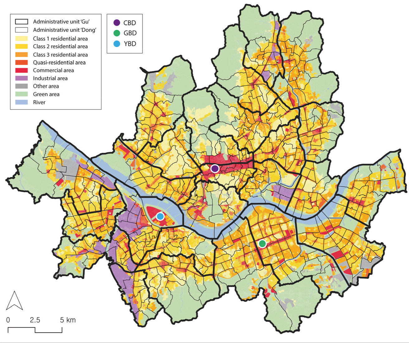
The total employment in Seoul is 4,574,965 [54], and the major employment centers are located in three areas: Jongno-gu and Jung-gu in the north (central business district; CBD), Gangnam-gu and Seocho-gu in the southeast (Gangnam Business District; GBD), and Yeouido and Yeongdeungpo-gu in the southwest (Yeouido Business District; YBD). Offices of major corporations and businesses are concentrated in these districts, which are designated as commercial areas due to their zoning for land use. Hence, approximately half of the total employment in Seoul is in these three districts [54].
Public transportation is active in Seoul due to congestion in the downtown area caused by the high population density. As of 2019, the modal split for weekday passenger cars was 24.5%, while public transportation accounted for 65.6% [55], indicating that a significant portion of travel within Seoul, including commuting, is conducted using public transportation.
Data
All The data on individuals’ commuting used in our study were derived from mobile phone data from 2019 provided by KT, the second-largest telecommunica-tions company in South Korea, accounting for approximately 25% of the country’s mobile phone subscribers [56]. The travel data were estimated based on communication between mobile phones and mobile communication base stations. Due to the extensive size of the dataset, we utilized data from one week, specifically from October 14 to October 18, 2019. During this period, the weather was clear, and it was an ordinary week without holidays or vacation periods, ensuring that typical daily travel patterns were present in the data.
As shown in Table 1, the data include the departure and arrival times (in one-hour intervals), the gender and age group of mobile phone subscribers, and the transportation polygon codes for both origin and destination locations. While our research focuses solely on commuting travels, the data do not indicate the purpose of travel. Instead, the origin and destination of travel are categorized as home, workplace, and other. This categorization is determined by the base station location, where communication by mobile phones during specific periods allows the estimation of daytime and nighttime stay locations. Consequently, these locations are categorized into assumed types, such as home and workplace. To identify commuting travels, we extracted samples meeting the following conditions: 1) travels where both the origin and destination are within Seoul, 2) travels that occur from 6:00 to 10:00, and 3) travels with home as the origin type and workplace as the destination type. These conditions consider the origin and destination types of travel as well as the typical commuting timeframes in South Korea. Through sample extraction, 2,016,347 samples from commuters were analyzed.
Table 1.
Examples of the information included in the mobile phone data
| ID | Origin (Departure) | Destination (Arrival) | Gender | Age | ||||
| Polygon code | Type | Time | Polygon code | Type | Time | |||
| 1 | XXXXXXX | H | 07 | XXXXXXX | C | 08 | M | 30 |
| ··· | ··· | ··· | ··· | ··· | ··· | ··· | ··· | ··· |
Methods
Variables
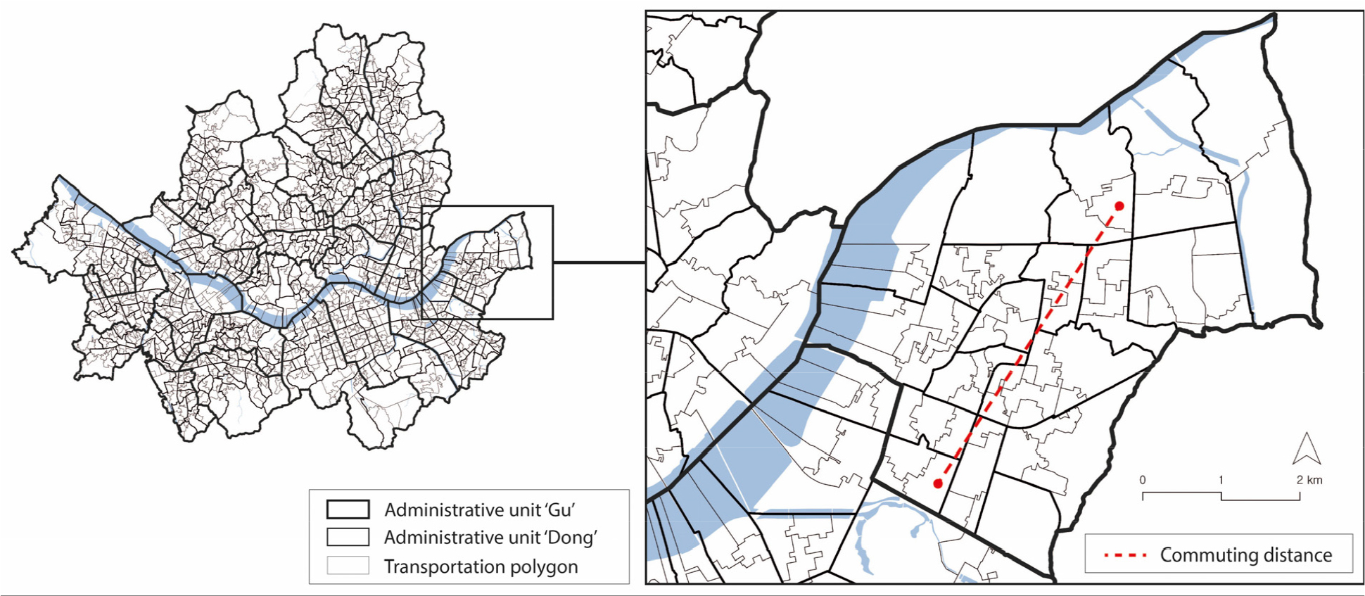
In mobile phone data, the origin and destination locations for each travel are provided at the transportation polygon level. Within Seoul, there are 1,785 transportation polygons, each with an average area of 0.34 square kilometers. As shown in Figure 2, the transportation polygon is much smaller than the administrative unit (‘dong’), which is the standard spatial unit of travel survey data. Therefore, we used transportation polygons as the spatial unit of analysis. The prediction target (i.e., the dependent variable), the commuting distance of each commuting sample, was calculated as the straight-line distance between the centroids of the origin and destination polygons.
The explanatory variables used to predict the commuting distance are listed in Table 2. Two socioeconomic factors (i.e., age group and gender of commuters) were derived from mobile phone data. Additionally, 12 built environment factors were constructed using variables frequently used in existing studies at the transportation polygon level.
Table 2.
Description of predictive variables
Population and employment densities are indicators that provide insight into residential and employment levels in each area. Research indicates that a higher residential density reduces commuting distance [9, 22], while commuting distances to high-density workplaces tend to be relatively longer [23]. Therefore, in our study, we aimed to verify whether the relationship between density and commuting distance differs between origins and destinations. Additionally, the relationship between density and travel distance may vary in East Asian cities compared with Western cities. Consequently, we also aimed to understand the impact of density on commuting distance, particularly in the densely populated city of Seoul, compared with Western cities. To construct these two variables, we used grid data (100m X 100m) of the population and employees. The population and employees were then summed for each transportation polygon, and density was calculated accordingly.
The land use mix (LUM) and job-population balance variables were constructed as diversity factors. To construct the LUM variable, we used building data categorized by building usage. Based on these data, we calculated the floor areas of residential, commercial, office, and industrial buildings within the transportation polygons. LUM was then measured by calculating the entropy index. The entropy index is widely used to assess the level of land use diversity [32] and is calculated as follows (Equation 1):
where is the proportion of the floor area ratio of building use to the total floor area ratio within the polygon, indicates the total number of building uses (in our study, 4: residential, commercial, office, and industrial). This index has a value between 0 and 1, where one indicates that the floor areas of buildings for the four uses within the polygon are mixed in equal proportions. Therefore, areas with a low LUM are primarily composed of a single land use, whereas areas with a high LUM have a balanced mixture of the four land uses.
Job-population balance was measured as the ratio of employees to the population within the polygon, serving as an indicator for job opportunities alongside diversity. Existing studies report diverse results regarding the impact of the job-population balance on commuting distance, necessitating additional empirical evidence [7, 57]. In particular, Boussauw et al. [48] and Peng [49] find that the job-population balance has a nonlinear relationship with travel distance. Therefore, we aimed to verify the relationship between job-population balance and commuting distance.
As a public transportation accessibility factor, a transit density variable was constructed based on the density of public transportation stops, including buses and subways. Public transportation accessibility at origin and destinations are significant variable influencing commuting mode choice. The use of automobiles is often associated with long-distance commuting; however, commuters heading to congested urban areas or CBD may opt for public transportation. Moreover, Seoul has a high share of public transportation. Therefore, public transportation accessibility at residences and workplaces may affect commuting distance by influencing the mode of transportation used for commuting.
Finally, as a destination accessibility factor, the distance to the CBD variable was constructed. Seoul has three major employment centers (CBD, GBD, and YBD). Therefore, we selected the most representative subway station for each employment center and calculated the straight-line distance between the centroid of each polygon and the closest subway stations. The representative stations for each employment center are listed in Table 2.
Design factors, which are included in the D variables were excluded from our analysis. Variables such as intersection density and street density are regarded as having a stronger association with mode choice than with travel distance. According to Ewing and Cervero [58], the elasticity of intersection density with respect to mode choice (e.g., walking and transit use) is greater than its elasticity with respect to VMT. As our study examines commuting distance, these design factors were excluded. However, future research incorporating these factors is warranted.
ML algorithms for the prediction model
To construct the prediction model, we selected three ML algorithms: Random Forest, LightGBM, and XGBoost. We compared their predictive performances and used the one with the best performance. All three algorithms are ensemble learning algorithms that generate predictions by creating and combining multiple learners. Ensemble learning algorithms are less sensitive to data and exhibit flexibility by combining multiple learners and averaging their results [18]. The prediction process proceeded as follows. For the commuting samples extracted from mobile phone data, we divided the data into training sets (70%) and test sets (30%). Subsequently, the GridSearch CV (cross-validation) function from the scikit-learn library (Python programming language) was employed to determine the optimal hyperparameters for each algorithm. Prediction models were then trained and validated using the hyperparameters. To evaluate the performance of each model, we used the mean absolute error (MAE) and root mean squared error (RMSE) metrics. The MAE signifies the average absolute value of the residuals, which are the differences between the predicted and actual values. At the same time, the RMSE represents the square root of the average of the squared residuals. Therefore, lower values for both metrics indicate higher prediction accuracy. Based on these metrics, we selected the model that demonstrated the best predictive performance.
XML techniques
To analyze the impact of the built environment factors observed during the commuting distance prediction process based on the final selected prediction model, we employed the SHapley Additive exPlanations (SHAP) technique. The SHAP technique, proposed by Lundberg and Lee [59], explains the prediction results by calculating the contributions of each variable based on game theory. It can capture both positive and negative relationships between the prediction target and explanatory variables, allowing for an understanding of the degree of impact through the SHAP values of each variable [10, 18]. We used the SHAP beeswarm plots for each variable to investigate the direction in which each variable contributed to the prediction of commuting distance.
However, the SHAP technique captures only the predictive contribution and direction of the impact of each variable. Therefore, to capture nonlinear relationships and other aspects not revealed by the SHAP technique, we conducted an in-depth analysis of the relationship between the built environment and commuting distance by generating a PDP. The PDP illustrates the marginal effect of a variable on the prediction target, controlling for the average effect of all other variables included in the prediction model [60]. By using PDP, we can comprehensively analyze the relationship between the prediction target and explanatory variables, identifying nonlinear relationships [10].
Results
Prediction model
The comparison results of the ML algorithms’ prediction performances are presented in Table 3. The average commuting distance for the entire commuting sample was approximately 7.05 km, with a standard deviation of 5.15 km. The results showed that the predictive power of ML methods surpasses that of linear regression models. Among the three ML algorithms, XGBoost had the highest predictive power, with an MAE of 1.2652 and an RMSE of 1.9080. In other words, based on the MAE, the XGBoost algorithm can predict an individual’s commuting distance with an error of approximately 1.3 km. Consequently, we constructed the final prediction model using the XGBoost algorithm, with the following hyperparameters: number of weak learners (n_estimators=1,000), learning rate (learning_rate=0.1), subsample ratio for data sampling (subsample=0.6), and the maximum depth of trees (max_depth=10).
Table 3.
Performance of prediction algorithms
| Model | MAE (km) | RMSE (km) |
| Linear regression | 3.7935 | 4.7601 |
| Random forest | 3.0293 | 3.9049 |
| LightGBM | 2.1599 | 2.9316 |
| XGBoost | 1.2653 | 1.9080 |
Descriptive statistics
Table 4 presents descriptive statistics for the socioeconomic factors. Individuals in their 30s are the largest group in the sample, followed by those in their 20s and 40s, while those aged 70 years and above are the smallest group. Regarding gender, while the proportion of male commuters in the actual population of Seoul residents is higher [61], females slightly outnumber males in our sample. This result might have been caused by commuters who reside in Seoul but work in other cities. Therefore, we might have missed male commuters traveling to other cities outside Seoul during the process of collecting the commuting sample within Seoul. Nevertheless, considering the large sample size and minimal difference in the gender ratio, we judged the likelihood of misestimation of the results due to sampling errors to be low.
Table 4.
Descriptive statistics for socioeconomic factors
Table 5 presents descriptive statistics for built environment factors. Each variable is constructed at the transportation polygon level. The average population density for each polygon is approximately 12,000 people per square kilometer. Employment density is like population density on average; however, due to the concentration of employment centers in certain areas, the standard deviation of employment density is significantly larger than that of population density. As expected in a city with an excellent public transportation system, each polygon has an average of approximately 27 public transportation stops per square kilometer, with some polygons having up to an average of around 172 stops.
Table 5.
Descriptive statistics for built environment factors
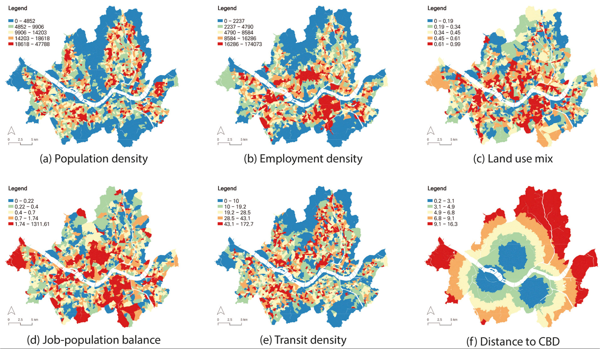
The spatial distribution of the built environment factors is shown in Figure 3. The spatial distribution categorizes variable values into quintiles, where the red and blue areas represent polygons with high and low variable values, respectively. First, the population density in Seoul (Figure 3a) appears to be higher in the outskirts than in the city center. This result can be attributed to the characteristics of Seoul. Seoul has numerous residential areas and new towns, composed of apartment complexes, distributed on its outskirts, resulting in a higher population density in these outskirt areas. Areas with low population density are correlated with high employment density (Figure 3b). Areas with high employment density align with the locations of the three major employment centers, as shown in Figure 1. LUM (Figure 3c) and job- population balance (Figure 3d) also show high variable values around employment centers and their surroundings. Moreover, considering the high level of active public transportation usage in Seoul, transit density (Figure 3e) is consistently high throughout the city. Areas with high population and employment densities exhibit similar levels of transit density. Finally, the distance to the CBD (Figure 3f), measured as the distance to the nearest employment center, naturally shows a concentric distribution around employment centers.
How the urban built environment affects commuting distance
Figure 4 shows the analysis results of the SHAP technique based on the commuting distance predictions generated by the prediction model using the XGBoost algorithm. The variable names prefixed with ‘O_’ denote characteristics of the origin (i.e., residence), while ‘D_’ represents characteristics of the destination (i.e., workplace). The order of variables in the figure indicates the importance of each variable observed during the prediction process. Each dot represents an individual data sample, with red dots indicating high variable values and blue dots indicating low variable values. The X-axis represents the SHAP value, with points positioned to the right and left of the baseline corresponding to high and low SHAP values, respectively. In other words, a distribution of red dots extending to the right of the SHAP value for each variable indicates a positive contribution to the commuting distance prediction. Conversely, an extension to the left signifies a negative contribution to the prediction.
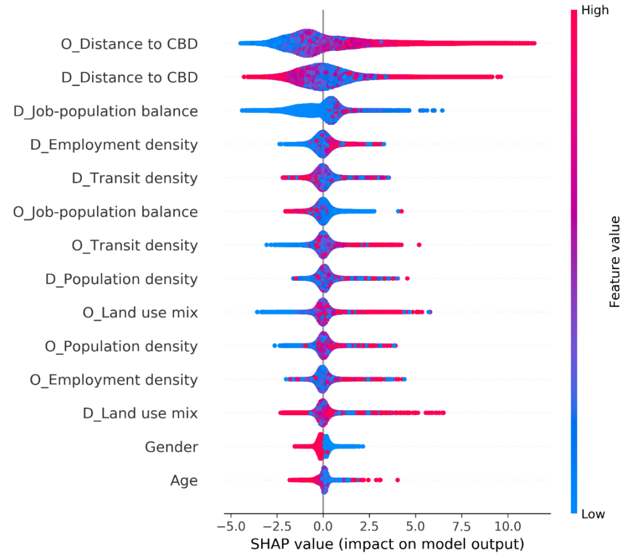
Overall, urban built environment factors are more significant than socioeconomic factors, with the distance from residence (workplace also) to the CBD being the most notable. These factors signify that the geographical location and accessibility of the residence and workplace are the most crucial factors in determining commuting distance. In particular, the distance from the residence to the CBD (O_Distance to CBD) is the most influential in predicting commuting distance, with a distinct distribution of red dots extending predominantly to the right. This result indicates a positive contribution to the prediction, implying that as the distance from the residence to the CBD increases, the commuting distance also increases.
Employment density at the workplace (D_Employ- ment density) also positively contributes to predicting commuting distance, indicating that the commuting distance to high-density employment areas is generally longer. This finding implies that similar to the interpretation of the distance from the residence to the CBD, a significant number of commuters heading to employment centers reside in outskirt areas.
Public transportation density at the residence (O_ Transit density) has a positive contribution to the prediction. This information suggests a preference for public transportation as a commuting mode, due to congestion resulting from high urban density in Seoul. Consequently, long-distance commuters are more likely to reside in areas with excellent accessibility to public transportation.
Regarding socioeconomic factors, gender exhibits a clear negative relationship with commuting distance, indicating that males have longer commuting distances than females. This finding aligns with the results of previous studies [39, 40]. Age appears to contribute negatively to commuting distance, although the presence of mixed red dots suggests that further investigation is required.
Nonlinear relationship between the urban built environment and commuting distance
The SHAP technique allowed us to confirm the contribution and direction of the impact of each variable. However, for variables where the red and blue dots are mixed, a nonlinear relationship could exist between these variables and commuting distance. Therefore, to comprehensively analyze this relationship and capture nonlinearity, PDPs were generated for each variable, as shown in Figure 5. The X-axis of the PDP represents the variable values. In contrast, the Y-axis represents the elasticity of commuting distance predictions. This finding can be understood as the change in the predicted commuting distance based on the variable values.
The variables that show a clear relationship in the SHAP analysis exhibit a consistent relationship in the PDP results. The results show that transit density at the residence (Figure 5e), distance from the residence to the CBD (Figure 5f), and employment density at the workplace (Figure 5h) have a clear positive relationship with commuting distance. Additionally, regarding gender (Figure 5n), females and males exhibit differences in commuting distances.
Population density at the residence (Figure 5a) displays a positive linear relationship with commuting distance; however, a detailed examination reveals a nonlinear relationship. As the population density at the residence increases, the commuting distance gradually decreases or remains constant. However, at the 90th percentile of population density, approximately 20,000 people/㎢, the commuting distance increases sharply. The employment density at the residence (Figure 5b) and job-population balance (Figure 5d) display similar forms of nonlinearity. Specifically, the job-population balance at the residence shows a negative slope, and the commuting distance is at its lowest when the value is approximately 1. However, when the variable value exceeds 1, the commuting distance also increases. The LUM at the residence (Figure 5c) displays a soft, U-shaped, nonlinear relationship. Similarly, the LUM at the workplace (Figure 5i) displays a nonlinear relationship. The results for both variables indicate that as the LUM increases, the commuting distance gradually decreases, reaching its lowest point near the average LUM value of 0.4. However, when the LUM exceeds this range, the commuting distance shows an increasing trend. This pattern suggests that very high levels of LUM at both the residence and workplace are associated with longer commuting distances.
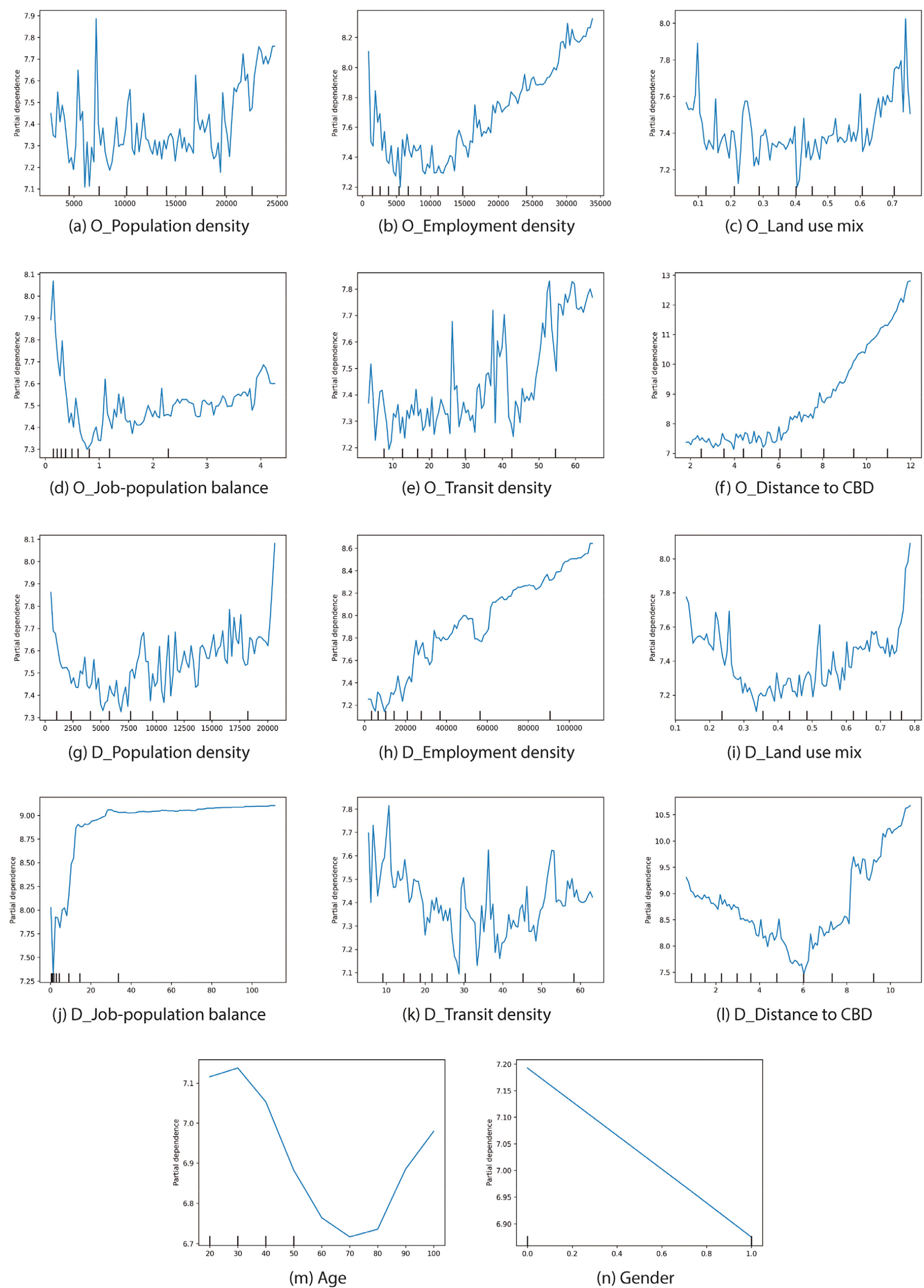
The job-population balance at the workplace (Figure 5j) displays a predominantly positive relationship, like the employment density at the workplace (Figure 5h). This indicates that commuting distances are longer for workplaces located in areas with high employment density and pronounced job–population imbalance. The transit density at the workplace (Figure 5k) displays a gentle U-shaped nonlinearity. The average transit density is approximately 27, and the commuting distance to areas with this value is the shortest. Commuters working in areas with poor public transportation accessibility tend to commute longer; however, as accessibility improves, commuting distances gradually decrease. Nevertheless, when the level of public transportation accessibility at the workplace increases significantly, commuting distances tend to rise again. Further, as the distance from the workplace to the CBD increases, the commuting distance gradually decreases, reaching its lowest point at an average distance of approximately 6 km and then increases again (Figure 5l). In other words, if the workplace is not in the CBD or outskirts, the commuting distance is the shortest. Conversely, if the workplace is in the CBD or far from it, the commuting distance increases.
Finally, from Figure 5m, as age increases, commuting distances gradually decrease. This decrease could be attributed to the limitations faced by younger commuters in choosing residences close to their workplaces due to the high cost of housing in the city center and CBD areas. As individuals age, they may have the option to choose residences in areas near their workplaces, resulting in shorter commutes. However, elderly commuters, particularly those aged 70 years and above, tend to have longer commuting distances, for reasons like those of younger commuters or considerations that arise after the typical retirement age.
Discussion and Conclusions
Our study aimed to examine nonlinear relationship between urban built environments and commuting distance in Seoul using XML techniques. To achieve this, we initially extracted individual commuting samples from mobile phone data and constructed a commuting distance prediction model using ML algorithms. The ML algorithms outperformed linear regression models, with the XGBoost algorithm showing the best performance. Subsequently, SHAP analysis was conducted to identify the impact of urban built environments on commuting distances, and PDP analysis was conducted to understand the inherent nonlinear relationships between built environments and commuting distances.
The results show that the distance from both the residence and workplace to the CBD is the most crucial determinant of commuting distance. The distance from the residence to the CBD positively contributes to the prediction, indicating that residents in outskirt areas tend to have longer commuting distances. This reaction by residents aligns with the findings of previous studies in other urban contexts [32, 33, 34]. Meanwhile, the distance from the workplace to the CBD exhibits a nonlinear relationship with commuting distances. Commuting distances are shortest when heading toward areas other than the CBD and outskirt areas. This reduced distance suggests that the geographical positioning of the city center and outskirts influences commuting patterns. Particularly in Seoul, which has densely populated residential areas in outskirt areas, many commuters heading toward the CBD face unavoidable long-distance commuting. Therefore, from a perspective of urban spatial structure, the creation of subcenters between the CBD and the outskirts can provide residents in the outskirts with closer employment opportunities, leading to an overall reduction in commuting distances within the city.
Population density at the residence exhibits a nonlinear relationship with commuting distances. Notably, when the population density exceeds a certain threshold, the commuting distance increases sharply. This finding suggests that the impact of density on commuting distance can vary across different urban contexts, contrary to the findings of numerous existing studies [22, 23, 24], which indicate that higher density tends to reduce commuting distances. Specifically, residents in the densely populated outskirts of Seoul may have a higher likelihood of undertaking long-distance commutes to the CBD, leading to the observed sharp increase in commuting distances with higher residential population density. In contrast, employment density at the workplace, as analyzed by the SHAP analysis, shows a positive relationship, indicating that higher employment density is associated with longer commuting distances. This determination aligns with the natural expectation that commutes towards the CBD, where employment is concentrated, tend to be longer, supporting the results by Manaugh et al. [23]. Since the impacts of density factors, especially residential population density, may vary across different study areas, further studies in diverse urban contexts are necessary to validate these effects and formulate context-specific urban policies.
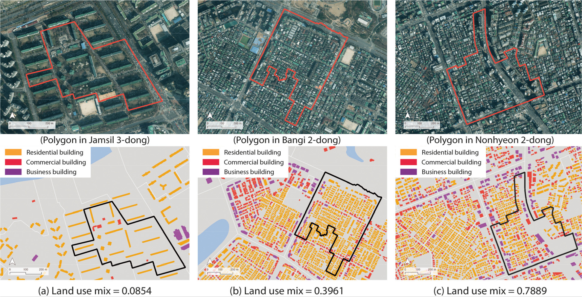
Additionally, while numerous studies have reported that a high LUM at the residence leads to a decrease in commuting distances [9, 28, 29], our study identified a nonlinear relationship between the LUM and commuting distances. The commuting distance is extended when the LUM at the residence is excessively low or high, while it is minimized when the LUM is around 0.3 to 0.5. These results can be attributed to the characteristics of the entropy index used to measure LUM. The entropy index attains its highest value of 1 when the four land use types are equally distributed. Consequently, areas with high LUM are presumed to be diverse commercial and business districts in city centers rather than typical residential areas. For instance, as illustrated in Figure 6, areas with a very low LUM are typically densely populated residential areas consisting of apartments, while areas with an LUM of approximately 0.4 represent regions where residential functions are appropriately mixed with other land uses. Conversely, areas with a remarkably high LUM are city centers characterized by the dense distribution of commercial buildings and offices. Therefore, in areas with very low levels of LUM, which are typically characterized as residential areas, residents may be unable to find job opportunities nearby, potentially resulting in longer commuting distances. Conversely, in highly LUM areas, residents may tend to commute to other functionally specialized city centers, which could likewise contribute to increased commuting distances. This nonlinear relationship highlights the role of appropriate LUM near residence in reducing individuals’ travel distances.
From the perspective of job-population balance, the commuting distance is shortest when there is a balanced ratio of population to employees residing in the area. This result supports the findings of existing studies [48, 49], which assert a nonlinear relationship between job-housing balance and commuting distance. In areas where the imbalance between the population and the workforce is severe, long-distance commuting is often inevitable to access employment opportunities. Conversely, a balanced ratio of population to employees near the residence can significantly reduce commuting distances. Therefore, strategies that can increase the accessibility between residences and workplaces are necessary to reduce individual commuting distances. This strategic outcome could be achieved through the formation of subcenters by physically bringing residences and workplaces closer together or by enhancing transportation networks that connect them.
Furthermore, better public transportation accessibility in residence, measured by transit density, is associated with longer commuting distances, consistent with previous studies [7, 36]. This finding suggests that long-distance commuters tend to choose areas with better public transportation accessibility as their residential locations, particularly in Seoul, where public transportation is the preferred mode of long-distance commuting. Meanwhile, transit density at the workplace has a nonlinear relationship with commuting distance, indicating that commuting distances to areas with either very poor or excellent public transportation accessibility are longer. Areas with poor public transportation accessibility are likely to be outskirt areas, whereas areas with excellent public transportation accessibility are likely to be city centers or CBD. This socioeconomic reality implies that commuters to workplaces in outskirt areas and the CBD have long commuting distances. These results may vary depending on the level of the public transportation system in each study area, making it difficult to generalize the variables’ impact. Nevertheless, in terms of urban transportation policies, our findings suggest that in areas with excellent public transportation systems, promoting public transportation usage as a mode of long-distance commuting can help mitigate environmental issues and congestion associated with private vehicle usage.
In terms of gender, commuting distances for males tend to be relatively longer, as reported in existing studies [37, 38]. This finding suggests that females may choose workplaces that are closer to their residences due to their household responsibilities. Regarding age, the commuting distance decreases with increasing age. However, for individuals aged 70 years and above, the commuting distance increases again. A probable reason is the high housing prices near the city center and the CBD. Therefore, to reduce commuting distances for these age groups, it is necessary to consider providing affordable housing near the city center or CBD, thereby expanding opportunities for residential selection.
Our study fill the research gaps by examining the nonlinear relationships between the built environment at the residence and workplace, as well as commuting distance in Seoul. Our findings indicate that the impact and direction of built environment factors revealed in existing studies may vary depending on the urban context. These insights can inform the formulation of customized strategies and policies, considering the unique characteristics of each city. Future research could use ML and other advanced techniques to conduct comprehensive analyses in various urban contexts, thereby accumulating a diverse body of empirical evidence.
Our study has the following limitations due to data constraints. We used the straight-line distance between transportation polygons as the commuting distance rather than the actual travel distance, which may not have fully represented the actual commuting experience. Additionally, due to privacy restrictions on mobile phone data, we were unable to consider information related to the mode of transportation. These limitations can be addressed in the future by collecting more comprehensive and specific big data that includes detailed and accurate travel information. Moreover, as the data were collected prior to the COVID-19 pandemic, our findings do not reflect post- pandemic changes in commuting patterns. Finally, future research should consider spatial autocorrelation, which was not explicitly addressed in our analysis.
