

Introduction
Literature Review
Machine Learning and Deep Learning Approaches in Basil Disease Detection
Transfer Learning Applications in Basil Disease Detection
Comparative Analysis of Studies
Materials and Methods
Transfer Learning
Datasets
Proposed Methodology
Hyperparameter Selection
Model Validation
Results and Discussion
Conclusion
Introduction
Agriculture is a necessity for the survival of mankind as it regulates and provides support to the food chain. In the past, farmers had to monitor crop growth manually by frequently visiting their fields. And crops were more tend to get affected by natural calamities and human error that leads to food shortage [1]. Thereby, traditional agricultural methods are vital to human life since they maintain and control the food chain. In the past, farmers relied on doing regular field trips to monitor crop progress, which frequently led to food shortages due to natural disasters and human error [1, 2]. Due to the remarkable amount of human effort involved, traditional agricultural methods are frequently less lucrative.
Deep learning which is a noteworthy subfield of machine learning and a proven effective approach for image classification task [3]. It shows marked success over various domains that also includes agriculture as well. Convolutional Neural Networks (CNNs) which contains specialized deep learning architecture can surpass in analysing images because of their inherent capability to independently obtain complex features from the unprocessed image data. These networks have shown its capability in the plant diseases classification by achieving high amount of accuracy and robustness [4].
The effective management of any vegetation with plant disease detection can increase the chances of urban ecosystem stability and plant life [5]. Agricultural productivity can be improved by using AI driven technologies which also helps in optimizing resource utilisation and emphasize on the usage of environmentally friendly practices [6]. Internet although is a valuable tool but to avail its maximum benefits for agriculture training is required [7]. Modernization and sustainability can go well together in spite of various contradictions using certain innovations, farmer centric methods and other policy supports [8].
Transfer learning is an approach where perception gained from a model by training it on a large dataset is applied to a related yet different task; has gained popularity in the field of deep learning. By using pre-trained models which uses already learned general image characteristics, transfer learning technique supports in significantly decreasing the amount of data required for training and quicken the training process, especially in situations with small datasets, which is very familiar in agricultural settings. In addition, transfer learning can often contribute to great performance as compared to building models from the scratch [9].
This research has its emphasis on benchmarking the seven pre-trained CNN models – EfficientNetB3, EfficientNetB2S, InceptionResNetV2, MobileNetV2, ResNet152V2, VGG16, and VGG19 – for the classification of basil leaf disease using two varied datasets. The model’s selection is done on the basis of their varying architectures, computational complexities, and proven performance in image classification tasks. The objective of this research is to use the efficiency of transfer learning in such situations to get the best model for accurate and efficient basil leaf disease detection. After comparing the performance of these models with different datasets, we target to provide valuable insights for developing practical disease management tools for basil cultivation.
The objective of this paper is to detect which dataset turns to be best for these pre-trained models which includes EfficientNetB3, EfficientNetB2S, InceptionResNetV2, MobileNetV2, ResNet152V2, VGG16, and VGG19. The main contributions of this work are as follows:
ⅰ.Comparative Analysis of CNN Models : The paper evaluates seven pre-trained CNN architectures (EfficientNetB3, EfficientNetB2S, InceptionResNetV2, MobileNetV2, ResNet152V2, VGG16, and VGG19) to determine their effectiveness in detecting basil leaf diseases.
ⅱ.Use of Two Distinct Datasets : The study employs two different basil leaf image datasets—one generalized dataset and one wild dataset—to assess the generalizability and robustness of the models under varying environmental and imaging conditions.
ⅲ.Performance Evaluation : The models are analyzed based on multiple metrics, including accuracy, precision, recall, validation accuracy, validation loss, and validation precision. The findings show that EfficientNetB3 performed the best on Dataset 1, while all models performed exceptionally well on Dataset 2.
The remaining section of this paper is organised as follows: Section 2 provides a review of prior studies on plant disease classification using machine learning and deep learning approaches. Section 3 explains the datasets utilised in this work, as well as the recommended technique, providing information on CNN architectures, the transfer learning process, and hyperparameter tuning. Section 4 presents the experimental results and discusses the performance of the different models. Finally, Section 5 concludes the article and discusses potential areas for further study.
Literature Review
This section reviews existing research on basil leaf disease detection and other related plant disease classification studies using machine learning and deep learning techniques.
As discussed earlier, Basil is a crucial herb that is commonly utilized in cooking, medicine, and agriculture. Yet, basil plants are prone to a range of diseases, including fungal infections, downy mildew, and Fusarium wilt, which can severely affect both yield and quality. Recent progress in machine learning (ML) and deep learning (DL) has made it possible to identify and classify plants disease with a high level of precision. Moreover, transfer learning—a method that makes use of pre-trained models—has enhanced the effectiveness of these approaches by building on existing knowledge from large datasets. This literature review examines the most recent studies on detecting basil diseases using ML, DL, and transfer learning. Here is a literature review of basil disease detection using ML and DL’s approaches, including the application of transfer learning, presented in a Table 1.
Table 1.
Statistical comparison of different techniques
| Study | Year | Title | Methodology | Dataset | Diseases Targeted | Performance | Transfer Learning |
| Rodríguez-Lira et al. [10] | 2024 | Trends in Machine and Deep Learning Techniques for Plant Disease-Identification: A Systematic Review” | Systematic review of ML and DL approaches for plant diseases identification | Several datasets across multiple plant species | Multiple plant diseases | Highlights effectiveness of CNN architectures like ResNet and MobileNet | Yes |
| Zhang et al. [11] | 2024 | Using Transfer Learning-Based Plant Disease Classification and Detection with a Novel IoT-Enabled Plant Health Monitoring System | Transfer learning with pre-trained CNNs; ensemble methods | PlantVillage dataset | Multiple plant diseases | Accuracy: 96.74% (early fusion), 97.79% (lead voting ensemble) | Yes |
| Mane et al. [12] | 2023 | Basil-Leaf Diseases Detection and Classification Using Modified Convolutional Neural Networks | Customized Convolutional Neural Network (CCNN) | 916 images of basil leaves | Fungiform, Downy mildew, Fusarium wilt, Healthy | Accuracy: 94.24% | No |
| Mane et al. [13] | 2023 | Basil Plant Leaf Disease Detection Using Amalgam-Based Deep Learning Model” | Hybrid model combining CNN using Support Vector Machine’s (SVM) and K-Nearest-Neighbor (KNN) | 803 images of basil leaves | Leaf spot, Downy mildew, Fusarium wilt, Fungal, Healthy | Accuracy: 95.02% | No |
| Kavitha et al. [14] | 2022 | Basil-Leaf Disease Detection Using Deep Learning Architectures” | Deep learning architectures for basil leaf disease detection | Images of basil leaves | Various basil leaf diseases | Performance metrics not specified | Yes |
| Alzubaidi et al. [15] | 2020 | Review of the State-of-the-Art of Deep Learning for Plant’s Diseases | Review of DL methods for plant disease detection | Various datasets | Multiple plant diseases | Discusses training, augmentation, and feature extraction methods | Yes |
| Dhingra et al. [16] | 2019 | Basil-Leaves Disease Classifications and Identifications by Incorporating Survival of Fittest Approach | Classification model employing an endurance of the suitable strategy and a 3-level hierarchical technique | Images of basil leave | Fungal, Downy mildew, Healthy | Detection rate: 95.73% | No |
The Table 1 summarizes recent studies focusing on basil disease detection using ML and DL methodologies, highlighting the datasets used, targeted diseases, performance metrics, and the applications of transfer learning methods.
Machine Learning and Deep Learning Approaches in Basil Disease Detection
Customized Convolutional Neural Network” (CCNN)
Mane et al. (2023) introduced a tailored convolutional neural network (CCNN) which was designed to find the diseases in basil leaves. Their research employed a dataset which consists of 916 basil leaves images and split them into four groups: healthy leaves, Fusarium wilt, downy mildew, and fungal diseases. The model attained an accuracy rate of 94.24% without using transfer learning. Their results focused the importance of deep learning for the initial detection of plant diseases, showing that larger datasets and data augmentation methods could additionally improve performance.
Hybrid ML Models: CNN with SVM and KNN
Mane et al. (2023) explored a hybrid method which combines convolutional neural network with the SVM and KNN. With the use of a dataset that contains 803 images of basil leaves, the model achieves an of 96.01% over five diversified categories of basil leaf diseases. The research focusses on the significance of both feature extraction and feature fusion approach for the improvement of classification accuracy. Nevertheless, it never includes the transfer learning method, which might increase the performance by manipulating knowledge from pre-trained networks.
Systematic Review of DL and ML in Plant Disease Detection
Rodríguez-Lira et al. (2024) did an in-depth examination of machine learning (ML) and deep learning (DL) methods for the identification of plant diseases, emphasizing on various plant species. Their results focused on the success of convolutional-neural-networks (CNN) like ResNet and MobileNet in the classification of plant diseases. The review also states the importance of transfer learning in improving model effectiveness, especially while working with smaller datasets. The study deduced that transfer learning plays highly important role in refining the model’s generalization across different species of plant.
Review of Deep Learning for Plant Disease Detection
Alzubaidi et al. (2020) inquired about various deep learning methods for recognizing plant diseases and found out that convolutional neural network (CNN) architectures such as VGG16, ResNet, and InceptionV3 have surpassed traditional machine learning methods in terms of accuracy and reliability. Their analysis has also given emphasis on the usage of data augmentation, feature extraction, and training strategies in improving deep learning models for recognizing plant diseases. The research came to the result that transfer learning significantly decreases computational expenses and training time while improving performance.
Transfer Learning Applications in Basil Disease Detection
Different transfer learning applications that have been mentioned in Basil disease detection are as follows:
Transfer Learning with Pre-trained CNN Models
Zhang et al. (2024) used transfer learning by balancing pre-trained CNN models for the classification of the plant diseases. With the usage of the PlantVillage dataset, their approach concluded an accuracy of 97.79% with the use of an ensemble of some pre-existing methods. The research spotlighted that using pre-trained architectures such as EfficientNet and ResNet reduces the need of extensive labeled datasets when improving the detection accuracy.
Survival of the Fittest Approach
Dhingra and colleagues (2019) devised a model for classifying various diseases in basil leaves by using a survival-of-the-fittest method. Their approach used a hierarchical classification technique and attained a detection rate of 95.73%. Although this method has a great potential but it lacked the inclusion of transfer learning strategies, which might have enhanced the model's applicability in other environmental contexts.
Deep Learning Architectures for Basil Leaf Diseases
Kavitha and colleagues (2022) surveyed the efficiency of various different deep learning architectures in identifying diseases on basil leaves. Their research highlighted the importance of using pre-trained models to increase the classification accuracy, especially in scenarios that involves limited datasets. Nevertheless, specific performance metrics were not detailed, resulting in complicating the comparisons with other research.
Comparative Analysis of Studies
Comparative analysis of various studies that were reviewed reveals various key insights as discussed below:
•Performance and Accuracy : Models using CNN-based architectures achieved high accuracy in a consistent manner, with transfer learning models outperforming traditional CNN models.
•Dataset Size and Quality: The productiveness of deep learning models depends majorly on the availability of the high-quality datasets. Transfer learning diminishes the issue of limited datasets by manipulating knowledge from pre-trained models.
•Hybrid Approaches: By combining CNN with traditional ML models such as SVM and KNN can increase feature extraction but also needs additional computational resources.
•Computational Efficiency: Transfer learning majorly reduces training time and computational costs and making it an appealing approach for real-world applications.
Materials and Methods
Various different materials and methods being used in this study is illustrated in this section. This paper presents the results on two distinct datasets after using seven different pre-trained deep learning models using transfer learning method.
Transfer Learning
Plant disease identification is an important constituent of precision agriculture, making it easy for early detection and intervention. This field has been transformed by deep learning, especially through transfer learning, which utilizes pre-trained convolutional neural networks (CNNs) in order to achieve high accuracy in plant disease classification. This methodology practices systems that have been developed on extensive datasets and alters them to particular agricultural needs. Various architectures, including EfficientNetB3, EfficientNetB2S, InceptionResNetV2, MobileNetV2, ResNet152V2, VGG16, and VGG19 are most commonly used because of their strong feature extraction capabilities.
EfficientNetB3 and EfficientNetB2S are a part of the EfficientNet series, being recognized for their efficient scaling techniques that can optimize depth, width, and resolution, making them to achieve high accuracy while still be computationally cost-effective EfficientNetB3's deeper structure permits it to grab more intricate features, whereas EfficientNetB2S is projected as a lightweight alternative that can be suitable for deployment in environments with limited resources.
InceptionResNetV2 combines the Inception module's parallel convolutional layers with the residual connections, improving convergence and reduces vanishing gradient problems. It is exceptionally adept at capturing features over varied scales, which is advantageous for differentiating between similar plant diseases.
MobileNetV2 is prepared as a lightweight model which is optimized for mobile and edge devices. The use of depth wise divisible convolutions reduces computational requirements while maintaining performance and making it suitable for real-time disease identification in the field settings.
Algorithm 1.
Plant Disease Classification
ResNet152V2, is a deep residual network that can handle the degradation challenge visible in very deep architectures by using identity shortcut connections. With a depth of 152 layers, it can easily learn highly abstract features, which helps in handling complex plant disease classification problems.
VGG16 and VGG19 are traditional deep CNN architectures distinguished by constant kernel sizes and a simple design. Even though they demand sufficient computational resources, they continue to keep significance because of their capability in extracting hierarchical features.
These models in transfer learning have to do pre-training on large datasets like ImageNet and are consequently fine-tuned for plant disease classification by deputing the classification head with custom layers. EfficientNet models generally outperform their counterparts about the accuracy and efficiency, whereas MobileNetV2 is generally favored for applications that requires real-time processing. The selection of a model is determined by considerations like the size of the dataset, handy computational resources, and the environment in which it is going to be deployed. With the use of transfer learning, plant disease classification can become more accurate and scalable, supporting farmers in initial disease detection and enhancing sustainable crop management. More description about this is mentioned in Algorithm 1.
Datasets
Two distinct datasets of basil leaf images were used in this study. Both datasets that are used are of distinct types. Dataset 1 is a generalized dataset and Dataset 2 is of Dataset in wild type. Images of both datasets are in .jpg format. Size of image in both datasets is 224*224*3. Sample images of both datasets are shown in Figure 1.
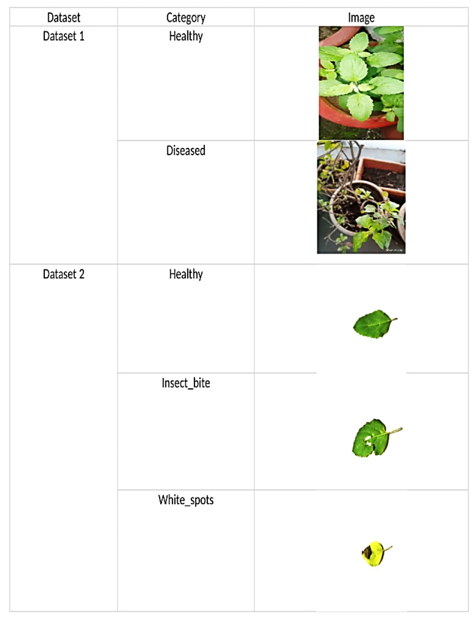
Dataset 1: Dataset 1 is a Basil leaf dataset collected from IEEE DataPort [17]. This dataset was published in 2019 and was last updated on 22nd December, 2020. This dataset is a generalized dataset which has a collection of images from Amravati, Pune and Nagpur regions of Maharashtra State from India. It has total of 1215 images. This dataset is further classified into 2 classes namely diseased and healthy. Diseased class contains 488 diseased images and healthy class contains 727 healthy images of Basil as shown in Table 2. Images are of dimension 3120*4160. The images have been resized to 75*75*3 where image size is 75*75 pixels with 3 color channels (RGB) to train ours model and meet deep learning model requirements.
Table 2.
Classes and number of leaves in Dataset1
| Dataset 1 | |
| Classses | Number of Images |
| Healthy | 727 |
| Diseased | 488 |
Dataset 2: Dataset 2 is a Basil leaf dataset collected from Kaggle [18]. This dataset is a type of Dataset in wild [19, 20, 21, 22, 23, 24, 25, 26, 27, 28, 29, 30, 31, 32]. This dataset has total of 12000 images. This dataset is classified into 3 classes namely healthy, insect_bite and white_spots; each of which contains 4000 images as shown in Table 3. Healthy class contains healthy Holy basil images, insect_bite contains images which illustrates various insect bite patterns and their effect on basil leaves, white_spots contains images depicting different manifestations of white spots and their impact on Holy Basil leaves. Images are of dimension 256*256. The images have been resized to 75*75*3 where image size is 75*75 pixels with 3 color channels (RGB) to train ours model and meet deep learning model requirements.
Table 3.
Classes and number of images in Dataset2
| DATASET 2 | |
| Classses | Number of Images |
| Healthy | 4000 |
| Insect_bite | 4000 |
| White_spot | 4000 |
Proposed Methodology
The proposed methodology, shown in Figure 2, applies transfer learning to seven pre-trained CNN models for basil leaf disease classification. Each model is fine-tuned to differentiate between healthy and diseased basil leaves using two diverse datasets.
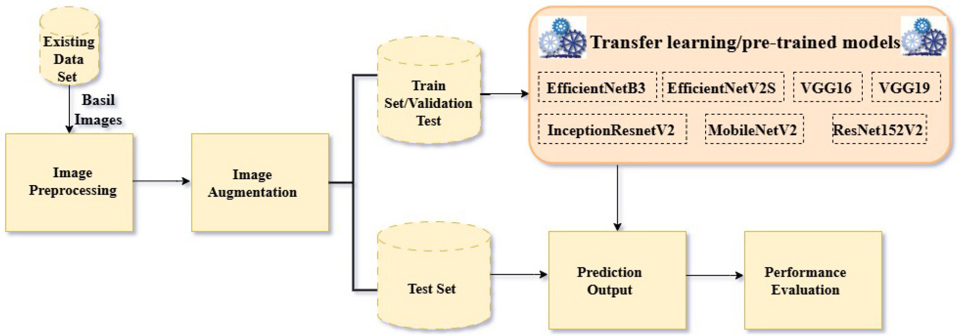
The classification model used is transfer learning as well as CNN. The steps involved are as follows:
1.Data Preprocessing: Images from existing dataset is processed by using rescaling, rotation_range, width_shift_range, height_shift range, shear range, zoom_range, horizontal_flip etc. where:
•rescale=1/255 which is used to normalizes pixel values to the range [0,1].
•rotation_range=20 which randomly rotates images by up to 20 degrees.
•width_shift_range=0.2 which randomly shifts images horizontally by 20% of the width.
•height_shift_range=0.2 which randomly shifts images vertically by 20% of the height.
•shear_range=0.2 is used to apply shear transformation with a shear intensity of 0.2.
•zoom_range=0.2 which randomly zooms in or out by 20%.
•horizontal_flip=True which randomly flips images horizontally.
2.Model Selection: Seven pre-trained CNN models were selected: EfficientNetB3, EfficientNetB2S, InceptionResNetV2, MobileNetV2, ResNet152V2, VGG16, and VGG19.
3.Transfer Learning: The pre-trained models were loaded, and the classification layers were replaced with new layers suitable for the specific number of disease classes in each dataset.
4.Training: The models were trained using the preprocessed datasets.
5.Evaluation: The performance of the trained models was evaluated using metrics such as accuracy, loss, precision, recall, validation accuracy, validation loss, validation precision, validation recall etc.
Hyperparameter Selection
Hyperparameter selection is crucial for performance in deep learning models. However, attaining optimal performance gradually depends on the careful selection of hyperparameters that includes learning rate, batch size, epochs, and network architecture choices etc. In our work, various hyperparameters are used such as image data generator hypermeters that includes rescaling etc., num_classes which has an assigned value of 2 for dataset1 and 3 for dataset 2. Model is set to 10 epochs which states that model iterated 10 times through the dataset during training. Few data generator hyperparameters that have been used, includes:
•x_col='image_path' which tells about the column in the dataframe that contains image file paths.
•y_col='label' tells about the column containing the class labels.
•target_size=input_shape[:2] → (75, 75) is used to resize images to 75*75 pixels.
•class_mode='categorical' states that labels are in categorical format (one-hot encoded).
•shuffle=True is used to shuffles data before passing it to the model.
•batch_size=batch_size → 8 tells about the number of images per batch.
The above hyperparameters have been applied to train_generator for training the data, valid_generator for validating the data and test_generator for testing the data. Few model’s architecture hyperparameters that have been used, includes:
•input_shape = (75,75,3) which informs about the input size of image for pretrained model e.g. EfficientNetB3.
•include_top=False is used to remove the fully connected layers from the model.
•weights=’imagenet’ uses already pre-trained weights from ImageNet.
•layer.trainable=False which is used to freeze all the layers in the pretrained model e.g. EfficientNetB3.
•GlobalAveragePooling2D() is used to replace the fully connected layer with the global average pooling (reduces overfitting).
•Dense(128, activation='relu') signifies a fully connected layer with 128 neurons and ReLU activation (number of neurons can be tuned).
•Dense(num_classes, activation='softmax') signifies that final layer for classification has 3 num_classes. The softmax activation function is used to convert the raw output values (logits) into probabilities that sum to 1.
Various training hyperparameters that have been used are:
•optimizer='adam' signifies that Adam optimizer is used which includes adaptive learning rate updates.
•loss='categorical_crossentropy' which is a loss function used for multi-class classification.
•metrics=['accuracy’] is used to track model performance using accuracy.
•epochs=10 is used to train model for 10 epochs (this can be tuned).
•batch_size=8 is used to determine the number of samples processed before updating weights.
Various evaluation and prediction hyperparameters that have been used are:
•test_generator.classes is used to extract the true labels from test data.
•Model.predict(test_generator) is used to generate the predictions.
•np.argmax(y_pred,axis=1) is used to convert probability outputs to predicted class labels.
•confusion_matrix(y_true, y_pred_classes): which is used to compute the confusion matrix to analyze misclassifications where y_true tells about true class labels from test_generator and y_pred_classes is used to predict class labels (converted from softmax outputs).
•classification_report(y_true, y_pred_classes, target_names=target_names)is used to generate a detailed classification report.
target_names=list(train_generator.class_indices.keys())is used to map numerical labels to their actual class names.
Model Validation
The seven pre-trained transfer learning models are used on two different datasets. The Dataset 1 is classified into 2 classes namely diseased and healthy. Diseased class contains 488 diseased images and healthy class contains 727 healthy images of Basil. Images are of dimension 3120*4160. The images have been resized to 75*75*3. The Dataset 2 is classified into 3 classes namely healthy, insect_bite and white_spots; each of which contains 4000 images. Healthy class contains healthy Holy basil images, insect_bite contains images which illustrates various insect bite patterns and their effect on basil leaves, white_spots contains images depicting different manifestations of white spots and their impact on Holy Basil leaves. Images are of dimension 256*256. The images have been resized to 75*75*3. The model was built using Keras and Tensorflow2.0 and used NVIDIA RTX 1650 as GPU for this experimental setup. Here 5-Fold Cross-Validation technique is used which is a resampling technique used to assess the performance of a deep learning model. The dataset is divided into 5 equal parts (folds), where the model gets trained on 4 folds and tested on the remaining 1-fold. This process gets repeated 5 times, each time using a different fold as the test set. The final performance is then obtained by averaging the results from all 5 iterations.
Results and Discussion
The results of the experiments are presented in this section. At first, results of Dataset 1 are discussed after applying transfer learning on these pretrained models which includes EfficientNetB3, EfficientNetB2S, InceptionResNetV2, MobileNetV2, ResNet152V2, VGG16, and VGG19 for basil leaf disease detection. Among all, the comparison is done on evaluated accuracies to find the best trained model.
For Dataset 1: EfficientNetB3 is the best pre-trained model for Dataset1 in case of transfer learning. Accuracy, precision and recall have been achieved with 94% and validation accuracy, validation precision and validation recall have been achieved with 99%. Table 4 below shows the results of dense neural network in case of Dataset1.
Table 4.
Baseline results with dense neural network for dataset 1
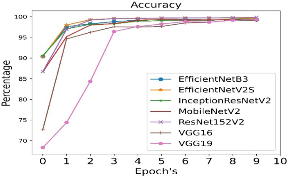
The accuracy is calculated for all seven pre- trained algorithms and is run for 10 epoch cycles. The highest accuracy is found to be achieved in case of EfficientNetB3 as shown in Figure 3.

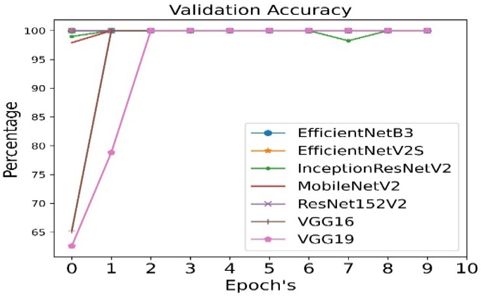
The validation accuracy is calculated for all seven pre- trained algorithms and is run for 10 epoch cycles. The highest validation accuracy is found to be achieved in case of EfficientNetB3 as shown in Figure 4.

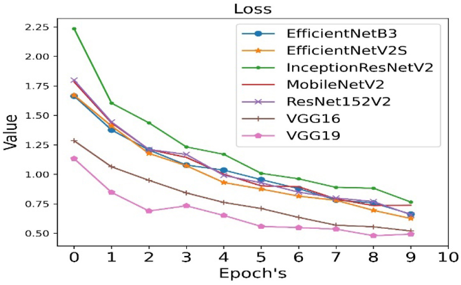
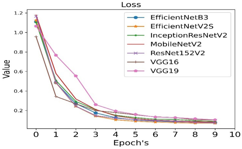
The loss is calculated for all seven pre-trained algorithms and is run for 10 epoch cycles. The loss is minimum in case of VGG19 as shown in Figure 5.
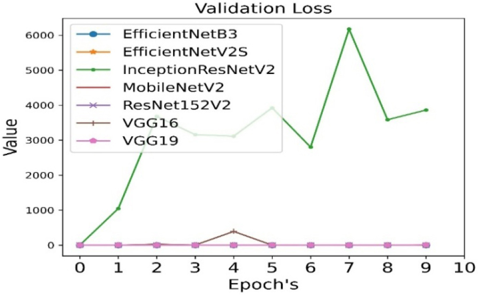
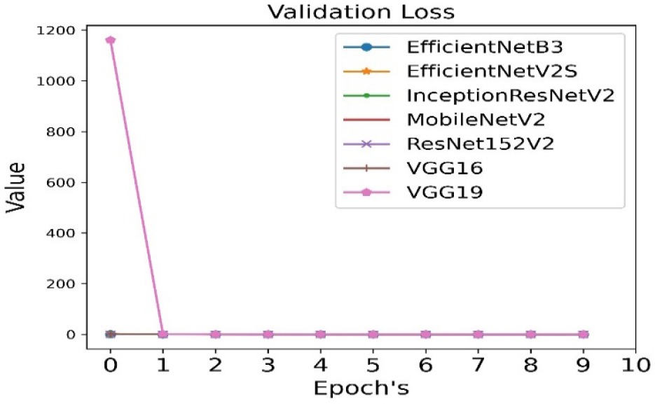
The validation loss is calculated for all seven pre-trained algorithms and is run for 10 epoch cycles. The validation loss is minimum in case of VGG19 as shown in Figure 6.
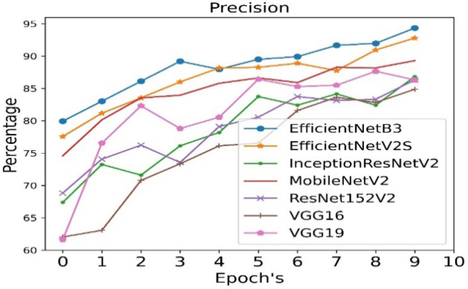
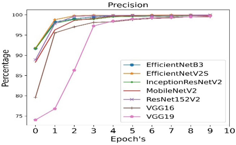
The precision is calculated for all seven pre- trained algorithms and is run for 10 epoch cycles. The highest precision is observed in case of EfficientNetB3 as shown in Figure 7.
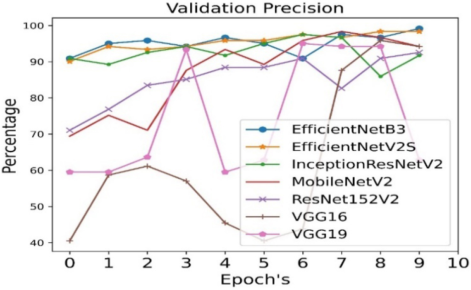
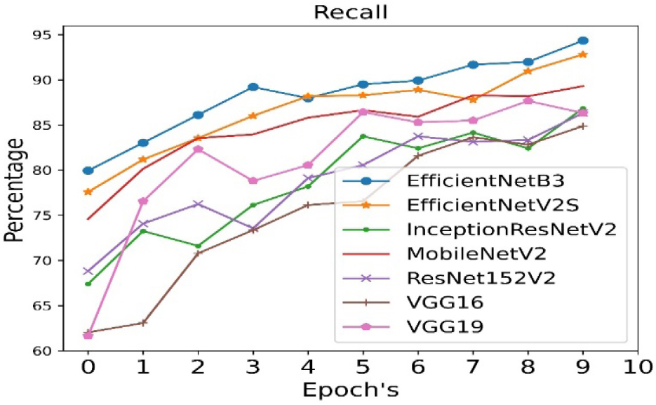
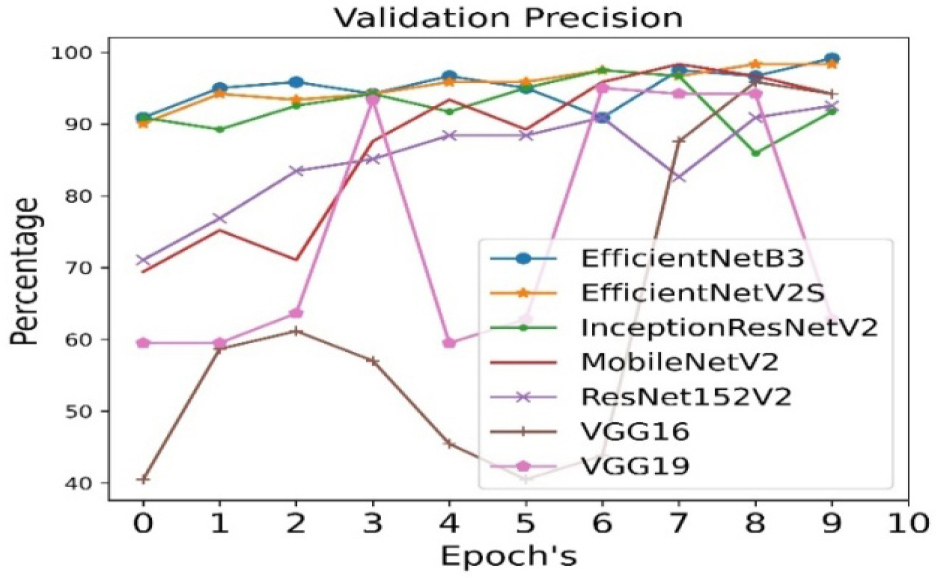
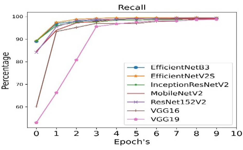
The validation precision is calculated for all seven pre- trained algorithms and is run for 10 epoch cycles. The highest validation precision is observed in case of EfficientNetB3 as shown in Figure 8. The recall is calculated for all seven pre- trained algorithms and is run for 10 epoch cycles. The highest recall is observed in case EfficientNetB3 as shown in Figure 9.
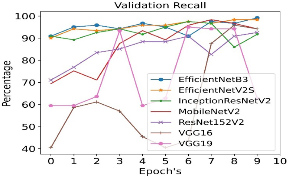
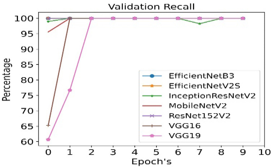
The validation recall is calculated for all seven pre- trained algorithms and is run for 10 epoch cycles. The highest validation recall is observed in case of EfficientNetB3 as shown in Figure 10.
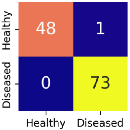
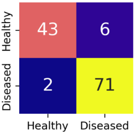
Confusion matrix gives a detailed evaluation of model’s classification performance by showing the correct as well as incorrect predictions for each class. The confusion matrix for EfficientNetB3 is shown in Figure 11.
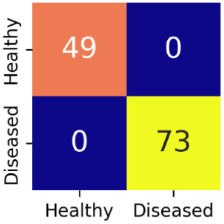
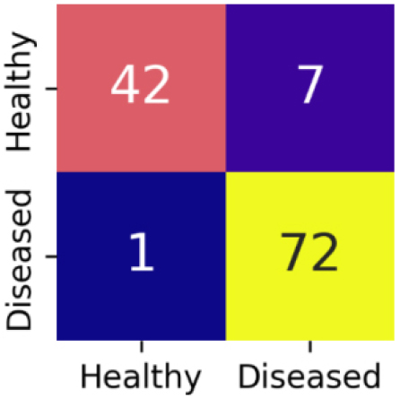
The confusion matrix for EfficientNetV2S is shown in Figure 12.
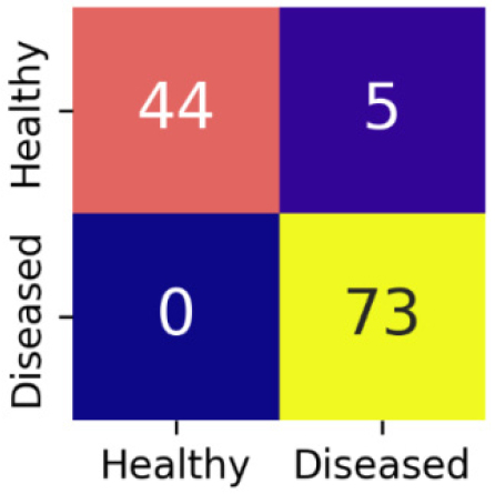
The confusion matrix for InceptionResNetV2 is shown in Figure 13.
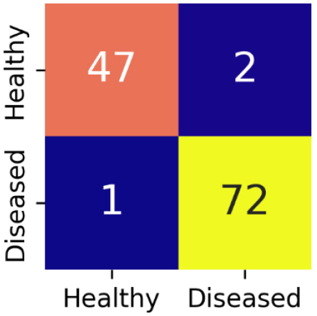
The confusion matrix for MobileNetV2 is shown in Figure 14.
The confusion matrix for ResNet152V2 is shown in Figure 15.
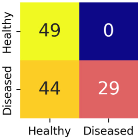
The confusion matrix for VGG16 is shown in Figure 16.
The confusion matrix for VGG19 is shown in Figure 17.
For Dataset 2: All models behaved well and given best results for Dataset 2 in case of transfer learning. Accuracy, precision and recall have been achieved with 99% and validation accuracy, validation precision and validation recall have been achieved with almost 100%. Loss and validation loss are not even 1%. Besides all algorithms work well in Dataset 2, Efficient NetB3 outperforms among them. Table 5 shows the results of dense neural network in case of Dataset 2.
Table 5.
Baseline results with dense neural network for dataset 2
The accuracy is calculated for all seven pre- trained algorithms and is run for 10 epoch cycles. Accuracy achieved on all seven pre-trained models is almost 99%. The highest accuracy with 99.86% is found to be achieved in case of ResNet152V2 as shown in Figure 18.
The validation accuracy is calculated for all seven pre-trained algorithms and is run for 10 epoch cycles. The highest validation accuracy is found to be achieved in case of EfficientNetB3 as shown in Figure 19.
The loss is calculated for all seven pre-trained algorithms and is run for 10 epoch cycles. The loss is minimum in case of EfficientNetV2S as shown in Figure 20.
The validation loss is calculated for all seven pre-trained algorithms and is run for 10 epoch cycles. The validation loss is minimum in case of EfficientNetV2S as shown in Figure 21.
The precision is calculated for all seven pre-trained algorithms and is run for 10 epoch cycles. The highest precision is observed in case of ResNet152V2 as shown in Figure 22. The validation precision is calculated for all seven pre- trained algorithms and is run for 10 epoch cycles. The highest validation precision is observed in all models as shown in Figure 23.
The recall is calculated for all seven pre- trained algorithms and is run for 10 epoch cycles. The highest recall is observed in case of EfficientNetV2S as shown in Figure 24.
The validation recall is calculated for all seven pre- trained algorithms and is run for 10 epoch cycles.
The highest validation recall is observed in case of all models as shown in Figure 25.
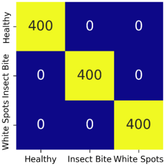
Confusion matrix gives a detailed evaluation of model’s classification performance by showing the correct as well as incorrect predictions for each class. The confusion matrix for all seven models is same as shown in Figure 26.
Conclusion
The results from both datasets highlight the impact of dataset diversity on model performance. Our findings indicate that models trained on wild datasets exhibit superior in-distribution accuracy, whereas those trained on generalized datasets demonstrate better robustness and adaptability to real-world agricultural applications. Specifically, for Dataset 1, EfficientNetB3 achieved the highest accuracy (94%), validation accuracy (99%), precision, and recall (94%). In contrast, for Dataset 2, all models performed exceptionally well, attaining 99% accuracy, precision, and recall across all evaluation metrics but Efficient NetB3 gave best results among them. So, Efficient NetB3 is the best algorithm in both the cases. These results underscore the importance of dataset selection in optimizing deep learning models for sustainable and resilient basil disease classification. This study reinforces the rapid developments in basil disease detection using machine learning, deep learning, and transfer learning. The integration of transfer learning techniques significantly enhances classification performance, making CNN-based models more efficient and reliable for real-world agricultural disease management. The effectiveness of these models across diverse environmental and imaging conditions highlights their potential for deployment in sustainable farming systems, especially in urban and precision agriculture settings.
Future research should focus on developing lightweight and computationally efficient models for real-time basil disease detection, ensuring scalability and accessibility for farmers with limited technological resources. The integration of IoT-driven smart agricultural systems could further enhance early disease detection, improving basil yield and quality. Additionally, exploring domain-specific data augmentation techniques and ensemble learning approaches may contribute to more robust and adaptive classification frameworks, fostering sustainable agricultural practices in both urban and rural farming environments.
