

Introduction
Literature Review
Data Analysis and Preprocessing
Dataset Description
Exploratory Data Analysis
Image Preprocessing
Image Segmentation
Methodology
Proposed Methodology
Hyperparameter Selection
Deep Learning Algorithms
Results and Discussion
Experimental Setup
Results for VGG-16
Results for VGG-19
Results for EfficientNetB0
Results for ResNet101
Conclusion and Future Scope
Introduction
Brain tumor refers to the pathological growth of cells that deviate from normal development, occurring either within the brain or in the adjacent tissues. The most prevalent kind of brain disease is a tumor. Brain is a most complicated component of human body and it is difficult for medical practitioner to detect brain tumor until patients start showing life-threatening symptoms such as seizures or memory loss [1]. The brain tumor type is determined by its size and location [2, 3]. Brain is broadly classified into benign (non-cancerous) and malignant tumor (vancerous). They can grow in any area of brain and are categorized depending on their location, size and cell type [4, 5].
Its treatment is determined by type, size and location. Radiation therapy, chemotherapy or Surgery, or combination may be used as treatment options. Meningioma is a non-cancerous tumor that is slow-growing tumors and consists of 85% of all tumor cases and forms into membrane which covers spinal cord and brain [6, 7]. These tumors can be surgically removed since they rarely spread to neighboring tissue. Whereas, pituitary tumors originate in pituitary glands, which are in charge of controlling the formation and function of hormones. Non-cancerous pituitary tumors hardly ever spread to other human organs. Malignant tumor cells are malignant cells that can infect nearby healthy tissues and develop abnormally and uncontrollably [8]. Gliomas is the most common malignant brain tumor which entails 33% of all type of tumors and approx. 80% of malignant brain tumors [7]. As per WHO guidelines, there are four grades of gliomas ranging from type I to type IV depending upon its size and location [9, 10]. Most people refer to Grade I and II as “benign” or low grade. Whereas Grade III (anaplastic astrocytoma) tumors are malignant and exhibit aberrant tissue morphology and Grade IV (glioblastoma multiforme) is the most severe stage of gliomas.
Clinical experts with skill in this field, for example, radiologists and particular specialists, review CT scans, X-rays, MRIs and PET scan pictures and decide a course of treatment on the basis of their findings [11, 12, 13, 14]. This process is tedious and requires many specialized skills. The identification, segmentation and localization of brain tumors with assistance of MRI pictures are troublesome and vital difficulties for automated computer applications [15, 16]. A deeper comprehension of the biology of brain tumors may result in the creation of novel diagnostic tools and strategies for detecting brain tumors earlier and more accurately.
The localization, segmentation and detection of tumors is difficult and a crucial challenge for medical practitioner and done mostly by gut feeling.
Main motivation of research, focusing on brain tumor detection, researchers can directly contribute to addressing a pressing healthcare need and positively influencing the lives of several people.
The integration of deep learning in medical science, especially in brain tumor detection, has changed the abilities of clinical diagnostics [17, 18, 19]. High level algorithms can now recognize patterns in clinical imaging that might escape from human detection, prompting prior and more exact tumor identification. The main contributions of this work are:
i. A comprehensive walkthrough on several DL methods and algorithms used for image classification, segmentation and detection.
ii.A detailed review covering Exploratory Data Analysis (EDA), performed on merged data set formed from four benchmarked data sets. Also includes steps taken on image augmentation including preprocessing and segmentation before classification model.
iii.To address this issue, deep neural network based architectures for multi classification were compared on four benchmarked datasets which are merged altogether for training & testing Deep learning model. The implementation of multi classification leveraging advanced deep learning based architecture are presented and detailed out the results on various performance and accuracy parameters.
The format of this document is as follows: The literature review presents application of deep learning models, analyses related work and identifies current research gaps. The dataset’s details, exploratory data analysis, image preprocessing methods like scaling and augmentation, and image segmentation for feature extraction are all covered under dataset description and exploratory analysis. The proposed methodology is described in the methodology section, along with hyperparameter tuning techniques and introduction of DL models (VGG-16, VGG-19, EfficientNetB0 and ResNet101). A comparison of deep learning algorithms, experimental configuration and outcomes utilizing performance metrics like accuracy and loss are presented in results and discussion. The findings are summed up, contributions are highlighted, limits are discussed, and new study directions are suggested in the conclusion and future scope section.
Literature Review
This section shows a list of recent studies in the field that is relevant to the topic by the author. In order to classify the MRIs into various classifications, Mohsen et al. [15] suggested a DNN classifier integrated with PCA and discrete wavelet transform. Fuzzy C-means clustering utilized for MRI image segmentation. However, model was performed on dataset having 66 brain MRI images. Abd-Ellah [20] suggested a unique two-phase multi-model automated diagnostic approach using VGG-16 and VGG-19. Overall accuracy of 94.85% on the test dataset. Sultan [21] suggested a deep CNN-based architecture for several brain tumor classifications, which involves dividing tumors into different groups and grading glioma tumors. The proposed approach bring accuracy of 96.13% and 98.7%, however model should be evaluated on a larger dataset. Sajid [22] proposed an approach for implementation of hybrid CNN architecture using patch- based method reflecting local and contextual data. Patch based approach was followed for segmenting Glioma tumor regions into two categories and no further classification was executed. However, model was performed on very small and single dataset. Chelghoum [23] proposed an approach to explain implementation of 9 pre-trained deep CNN networks like VGG16, ResNet18, GoogleNet, ResNet101, VGG19, SENet, ResNet50 and ResNet-Inception-v2 for classification of brain tumor. Badža [24] proposed an approach based on deep CNN classifying tumor into 3 distinct categories. For additional assessment, a cross-validation technique has been applied to both the original and enhanced photos. Naser [25] performed U-Net segmentation on tumor affected areas and developed deep VGG-16 model to grade Gliomas tumors. However, very small dataset has been utilized for validation and no independent grade data set available to compare. Kwabena [26] explained scenarios, having limited dataset for training and testing. CNN architectures often require a huge dataset for training data and its effective prediction. CNNs typically lower image resolution when processing to the hidden layer, resulting in a drop in classification accuracy. To overcome this challenge, author proposed CapsNets. CapsNets brings many advantages over CNNs, such as reducing feature loss via pooling and maintaining spatial information which helps in faster training and better accuracy. Deeksha [27] enhanced efficiency and accuracy of diagnosis, it proposes CNN model for classification of brain tumors. The model underwent initial training using a huge dataset of labeled pictures, following which it can classify any given MRI image to accurately categorize type of tumor. The model achieves accuracy of 92.62%. Irmak [11] put forward an approach for multi classification using deep CNN based architecture leveraging grid search optimizer. Three DCNN models were developed for three classifications of brain tumor. The accuracy of second classification model, which was developed to categorize tumors into several types, was 92.66%. Ayadi [28] proposed CNN model using 3 public datasets. Rembrandt, Figshare and Radiopaedia datasets were used for classifying tumor into three categories. Kevin [29] utilized brain tumor staging and anatomical phenotyping. In the study, brain tumor patients’ MRI images were analysed, and a new approach was created for classifying and staging these tumors according to their anatomical characteristics. The study’s findings demonstrated the potential use of anatomical phenotyping and staging as a tool for estimating the prognosis and course of treatment for individuals having brain tumors. Muhammad [30] utilized a DL-based decision support system to facilitate the brain tumors classification across multiple modalities. The DenseNet201 Pre-trained model has been used. There were two techniques, Entropy–Kurtosis based features selection and Modified Genetic Algorithm based features selection. Model classified brain tumors using several modalities with great precision with an overall accuracy of over 90%. Khan [31] introduced two CNN models based on deep learning techniques for classifying binary (normal -non tumor and abnormal - tumor) and type of tumor. The author constructed a 23-layer CNN model for tumor identification. To enhance classification job, transfer learning was employed with the help of the VGG16 architecture and adaptation of the initial CNN architecture presented by the author. Models gives up to 97.8% accuracy for deduction and 100% classification accuracy. Akter [32] proposed data merging technique, four individual datasets were combined to make two new merged dataset, which finally used for multi classification and segmentation. Model demonstrate high classification accuracy of 98.7% and 98.8% with the segmentation. Agarwal [33] suggested image augmentation technique to improvise the dataset for training & testing. Two CNN models were used to determine if an MRI was malignant or not, and a second model was used to determine the type of tumor- gliomas, meningiomas, and pituitary tumours. Kordnoori [34] used two distinct datasets. The first was of Nanfang Hospital from 233 patients which includes T1-weighted contrast- enhanced images comprising 3 types and second dataset covers Glioma Grades (HGG, LGG). A single segmentation decoder, a shared feature representation encoder and a multi-layer perceptron for meningioma, glioma, and pituitary adenomas classification are all included in the models.
Data Analysis and Preprocessing
A thorough summary of the dataset and the preliminary analysis done to obtain insights is given in this part. Using statistical techniques and visual aids, exploratory data analysis (EDA) was carried out to comprehend structure of the data set, spot trends, and find any abnormalities or outliers [35, 36, 37]. Image preprocessing techniques such as scaling, normalization, and augmentation are used to improve image quality and prepare data for deep learning models. In order to identify pertinent areas within the images and enable more precise feature extraction, image segmentation was finally used. These actions are essential to guaranteeing strong model performance in later phases.
Dataset Description
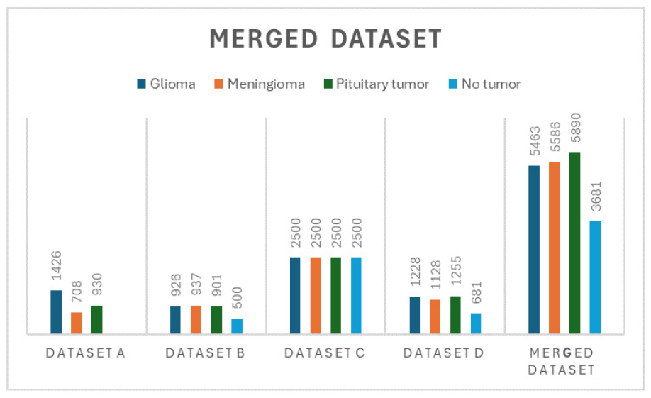
Four individual benchmarked datasets consisting of dataset a, b, c, d are used and formed one merged data combining all four individual datasets, follow appending one by one after removing redundant MRI images into merged Dataset. Merged dataset is finally used for preprocessing and classification Model development post image augmentation. Merged dataset involves the process of appending images and the combined directories, ensuring a comprehensive and unified dataset for further analysis.
•Dataset a - Dataset a is picked from Nanfang Hospital in Guangzhou, China, and General Hospital, Tianjin Medical University, China. This is widely used in many research papers and made publicly available by [38]. The images were captured using a type of MRI technique called spin-echo-weighted imaging, which provides detailed images with a resolution of 512 × 512 pixels [28, 39, 40]. MRI Images broken into three categories of Tumor - Glioma (1426), Meningioma (708) and Pituitary tumor (930) from 233 patients.
•Dataset b - Dataset b comprises of identical 3264 T1, T2 and fluid-attenuated MRI images and made available by [41]. For this dataset, the authors referred to a study about accurately detecting brain tumors using deep CNN network. Dataset split into training and testing. Testing directory includes pituitary (74), meningioma (115), glioma (100), and no tumor (105). Training directory consists of pituitary (827), meningioma (822), glioma (826), and no tumor (395).
•Dataset c - Dataset C consists of 10000 MRI images and entire data split into training, testing and validation. This dataset made available by [27]. Dataset is broadly classified all MRI images into 4 classes - meningioma (2500), pituitary (2500), glioma (2500), and no tumor (2500).
•Dataset d - Dataset d consists of 4292 MRI images and made available by [42]. In this particular dataset, the authors have taken a reference from [31, 33]. This dataset divided all MRI pictures into training and testing directories, and each of these directories contained meningioma, glioma, pituitary, and no tumor.
•Merged Dataset - Merged dataset involves appending all images from each dataset and the combined directories, ensuring a comprehensive and unified dataset for Model development.
Four distinct datasets: a, b, c, d was appended to one & after to formed merged dataset to keep only identical images as represented in Figure 1.
Exploratory Data Analysis
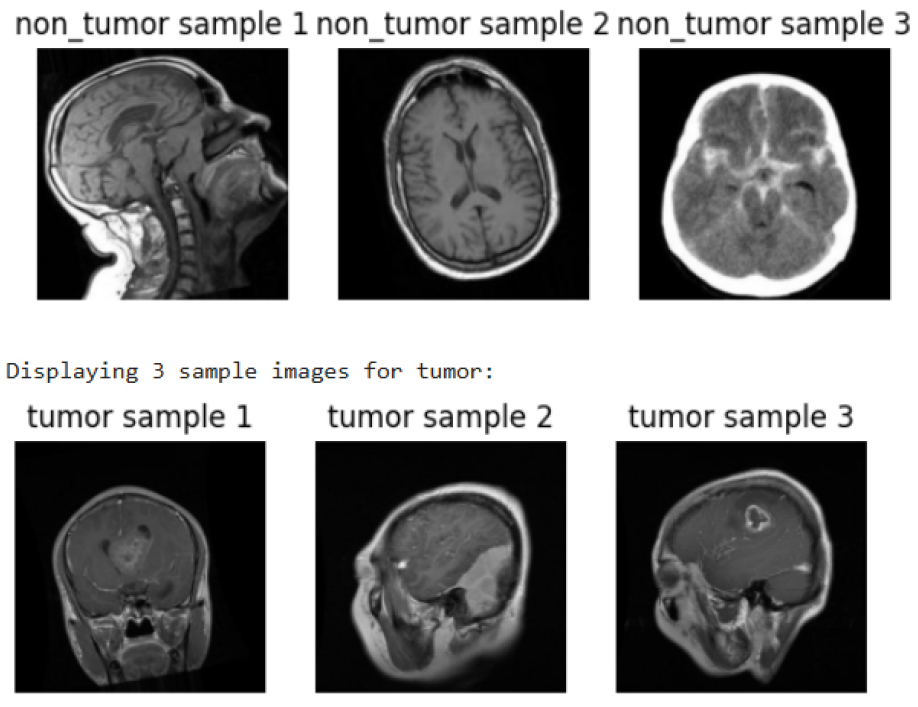
The collection consists of 3,681 samples without a tumor label and 16,939 samples with a tumor identification. Figure 2 shows sample MRI scans sorted into two groups: tumor (bottom row) and non-tumor (top row). To aid in the differentiation of tumors from healthy brain tissues in medical imaging, each category has three illustrated cases that demonstrate the visual distinctions in brain structures for both conditions.
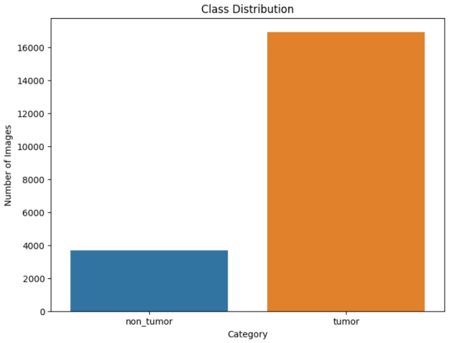
The class distribution of dataset is depicted in Figure 3. With 16,939 shots identified as tumors (orange) and only 3,681 photos classified as non- tumors (blue), there is a significant gap. This disparity highlights the need of approaches for controlling unbalanced datasets during model training in order to make accurate predictions.
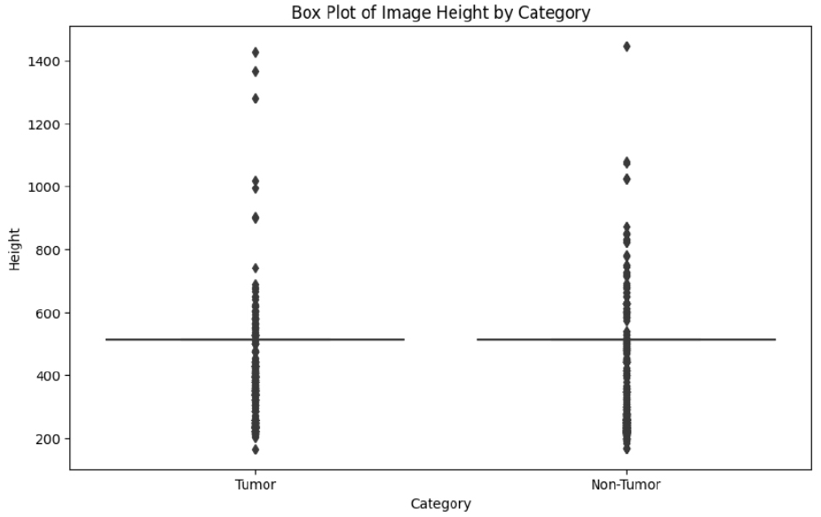
The box plot shown in Figure 4 indicates comparison of heights of images in “Tumor” and “Non- Tumor” categories. Both distributions share the same value around which their median heights exist. There are many outliers towards the higher end, indicating there is variability of image heights. The spread throughout both categories appears to be constant, meaning that there are not extreme height differences between them.
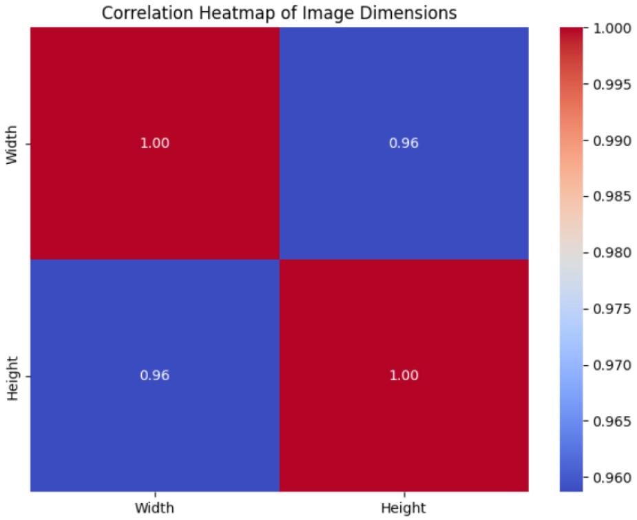
This heatmap in Figure 5 illustrates the connection between image width and height. The diagonal shows perfect correlations (1.00) since variables are compared to themselves. The off-diagonal value (0.96) indicates a significant positive correlation, suggesting that aspect ratios are consistent across images and that height tends to increase in proportion to width.
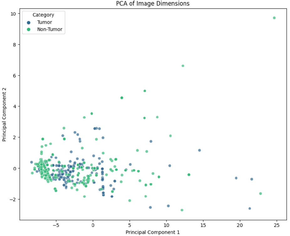
Images are categorized into “Tumor” and “Non- Tumor” categories in this scatter plot, which displays the findings of Principal Component Analysis (PCA) for picture dimensions. Points indicate reduced- dimensional representation, and some points overlap which indicates related features. The dispersion along Principal Component 1 highlights greater variance, whereas outliers imply unique visual characteristics. PCA facilitates the visualization of patterns of difference between groups as shown in Figure 6.
The two class’s imbalance highlights how important it is to manage class differences during model training in order to increase prediction accuracy. Principal component analysis, correlations, and picture dimensions all reveal recurring patterns in the collection, while a few outliers point to the existence of distinctive image features. These results offer a strong basis for additional modeling and preprocessing methods, like data augmentation and balancing tactics, to improve tumor classification models’ performance.
Image Preprocessing
Each original images has undergone to preprocessing steps consists of applying 9 different augmenting techniques on each image [43]. Image augmentation techniques includes Horizontal flip, Vertical flip, rotation, Adjustment on Brightness, resizing & zooming, Filtering like mode & sobel filter, grayscale conversion, unsharp masking, and & noise addition are added to make 9 times of original dataset.
MRI scan augmentation involves modifying images by adjusting orientation, size, appearance, and adding variations to enhance model robustness and generalization as shown in Figure 7. Nine augmentations techniques were applied on merged dataset of 20,690 original MRI images to create the 185,580 improvised images.
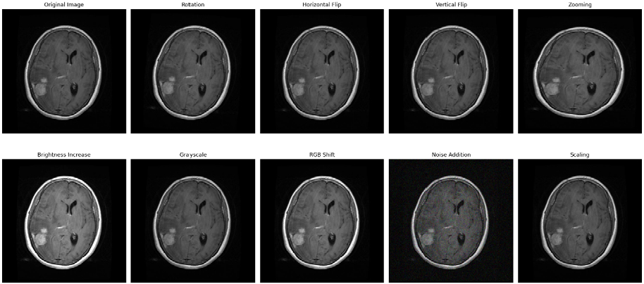
Image Segmentation
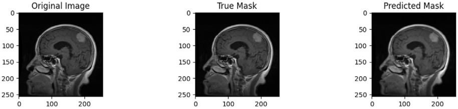
Four distinct datasets are appended to form the merged dataset which is finally used for model development. A masked dataset is used to train the segmentation model. Figure 8 display original images, true masks and predicted masks. The original brain MRI picture, the anticipated segmentation mask and the real segmentation mask are contrasted in this image. The real mask shows the ground truth region of interest, whereas the predicted mask shows the model’s output. The comparison shows that the model can accurately identify the target area.
Methodology
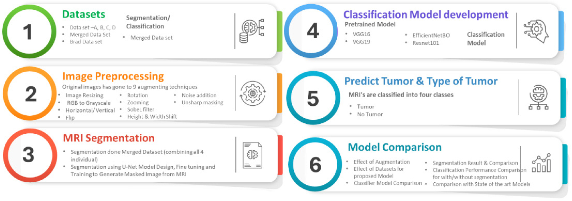
This section explains the step-by-step methodology followed for tumor classification as shown in Figure 9. Four distinct datasets were appended to formed merged dataset/directory. Finally merged directory which combining MRI images from all four datasets was used for segmentation and classification model.
This helps AI models to have enough MRI images for training and testing. There are multiple performance metrics used to comparing performance of multiple deep learning model and then gives best accuracy and performance.
Proposed Methodology
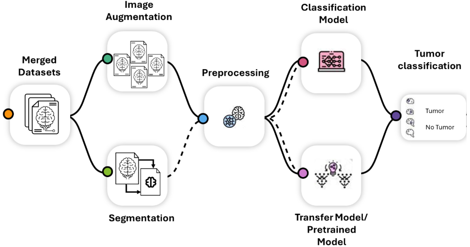
A step-by-step workflow for classification of MRI tumors using ML is depicted in Figure 10. Creating the dataset by combining labeled data for segmentation and classification is the first step. Image pre- processing uses augmentation techniques including noise addition, scaling and flipping to improve quantity of data. In MRI segmentation, U-Net carries out accurate pixel-wise labeling, separating various tissue types, such as tumors. Rather than simply detecting areas of interest, U-Net segments the image by labeling each pixel with a category, essentially outlining tumor boundaries and other structures for proper medical analysis.
Pre-trained models such as VGG16, EfficientNetB0 and ResNet101 are used to improve dataset for classification. These models are capable of classifying MRI scans as either tumor or no tumor. The models’ performance is then evaluated by contrasting them with the most advanced models and assessing the effects of augmentation and segmentation. Merged directory was formed from four distinct datasets and then merged dataset was taken for preprocessing including applying various techniques of image augmentation to make merged datasets multiplied by 9 times before passing it for segmentation and followed by classification. This process guarantees accurate and reliable tumor identification for medical imaging applications.
Hyperparameter Selection
Hyper parameters act as adjustable controllers while training deep learning model. To systematically optimize model performance, hyperparameter tuning comprises iterative adjustments that use methods such as random search, grid search and Bayesian optimization [44]. To achieve the best results, the optimal values for these hyperparameters are determined. Model hyper parameters include Input and output activation functions, optimizer function, loss function, batch size, no of epochs are given in Table 1.
Table 1.
Hyperparameters selected for classification model
Deep Learning Algorithms
Deep learning-based model architectures can handle enormous amounts of medical pictures efficiently, as they have become increasingly popular in medical imaging and diagnostics, extracting features, pattern accurately to deduct and segment tumor accurately [45, 46]. DL methods have been widely employed for image processing, classification, segmentation, detection and prediction as the number of large-scale, authentic labelled medical datasets with GPU computation capacity has grown. CNNs provide cutting-edge performance, particularly in the medical imaging area, as they can process, learn and extract features and patterns from MRIs and CT scans.
The fundamental CNN design consists of numerous layers, including convolutional, pooling, activation and fully linked layers. In order to extract features like forms, edges, and textures, convolutional layers use filters [47]. Pooling layers down samples the image to reduce computation, thus helping the network to generalize. Layers at the network’s end that are fully connected map learned features to the final prediction. Basic CNN architectures may not always capture complex patterns in medical images, particularly when the data is limited or highly heterogeneous. CNN based DL algorithms are emerging as a powerful tool for image classification and segmentation. A multi classification model has been proposed and evaluated on merged datasets formed using four benchmarked individual datasets. A segmentation approach was suggested which takes MRIs as input and creates masked pictures before classification of tumor to improvising the deduction accuracy.
Several advanced CNN deep learning based architectures designed to address limitations of basic CNNs model in improvising performance in medical imaging tasks [48, 49, 50, 51].
•VGGNet - VGGNet is called for its simple and uniform architecture, using smaller convolutional filters (3x3) stacked together to increase the depth of the network. VGG-16 model was pre-trained on a huge image dataset to discover intricate features useful for brain tumor image classification. Consequently, the model has demonstrated success in classification tasks, with high tumor discovery accuracy. VGGNet’s deep architecture with small filters captures fine-grained details in medical images. It is also relatively easier to implement and fine-tune.
•ResNet - With the introduction of residual learning, ResNet enabled it for networks to be much deeper without experiencing the vanishing gradient issue. ResNet allows connection to skip one or more layers without affecting overall performance. This technique aids in shielding the network from the gradient issue. Its architecture may vary, but it contains a series of residual blocks followed by fully connected layers. The residual connections in ResNet allow for training of extremely deep networks, improving performance in complex tasks. It is particularly effective in learning from large-scale medical imaging datasets. Despite its advantages, ResNet can be computationally expensive, and its deep architecture may not always be necessary for simpler tasks.
•EfficientNet - EfficientNet is a deep CNN architecture built upon a concept called “compound scaling” that equivalently scale width, depth, and resolution to provide high accuracy. This architecture optimizes the balance between accuracy and computational efficiency by scaling parameters. Scalable: You can choose a model variant (e.g., EfficientNet-B0 to B7) that best suits your computational resources and accuracy requirements.
Results and Discussion
The experiments broadly classified into individual model results and model performance comparisons. A total of four labeled datasets were used for forming merged directory which was later used for training and testing. Four deep CNN models are trained and evaluated.
Experimental Setup
Both personal PCs and cloud services, such as Google Collab, have been used in the project. The experiment’s broad scope involves developing & evaluating multiple deep neural networks and transfer learning model on diverse classification and segmentation datasets. There are various libraries such as Numpy, Tensorflow, Sklearn etc and several packages are used while developing ML model.
Results for VGG-16
VGG-16 is pre trained on huge medical imaging dataset and allows learning complex features and pattern that are useful for classifying and deducting brain tumor. Hence, VGG -16, a deep CNN have been applied to detect brain tumor. VGG 16 model’s training accuracy was 0.9936 with a training loss of 0.0204, its validation accuracy was 0.9851 with a validation loss of 0.0543. Figure 11(a) shows the accuracy in training and validation over epoch. While training accuracy steadily rises to a peak of almost 99%, validation accuracy varies widely. Because it suggests overfitting, shows model performs good on training data but inconsistently on validation data, this variability suggests potential issues with generalization.
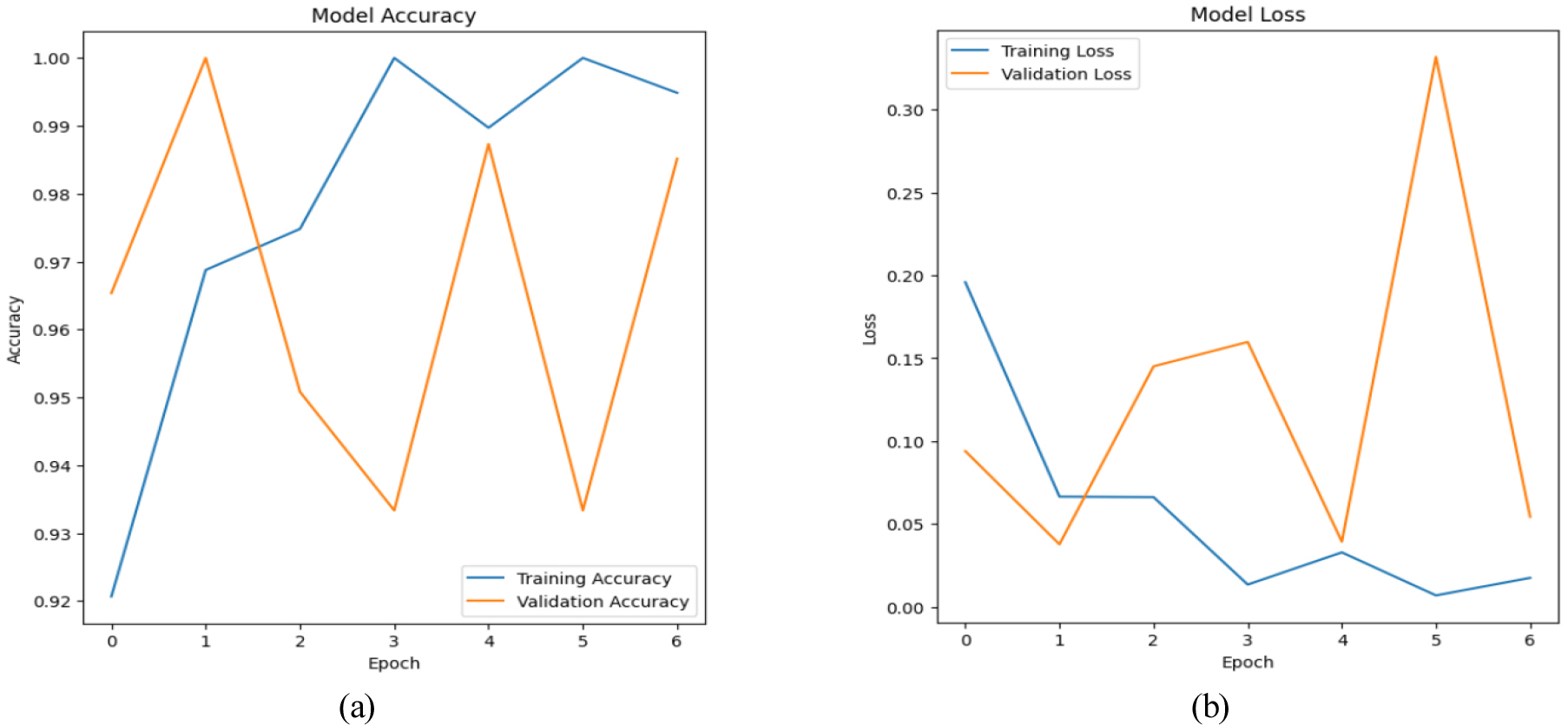
The validation and training loss of a model over time is shown in Figure 11(b). Learning is indicated by a steady decrease in training loss. However, validation loss fluctuates and peaks around epoch 5, suggesting overfitting or instability. The difference in losses indicates that training data performs better for model than unobserved validation data.
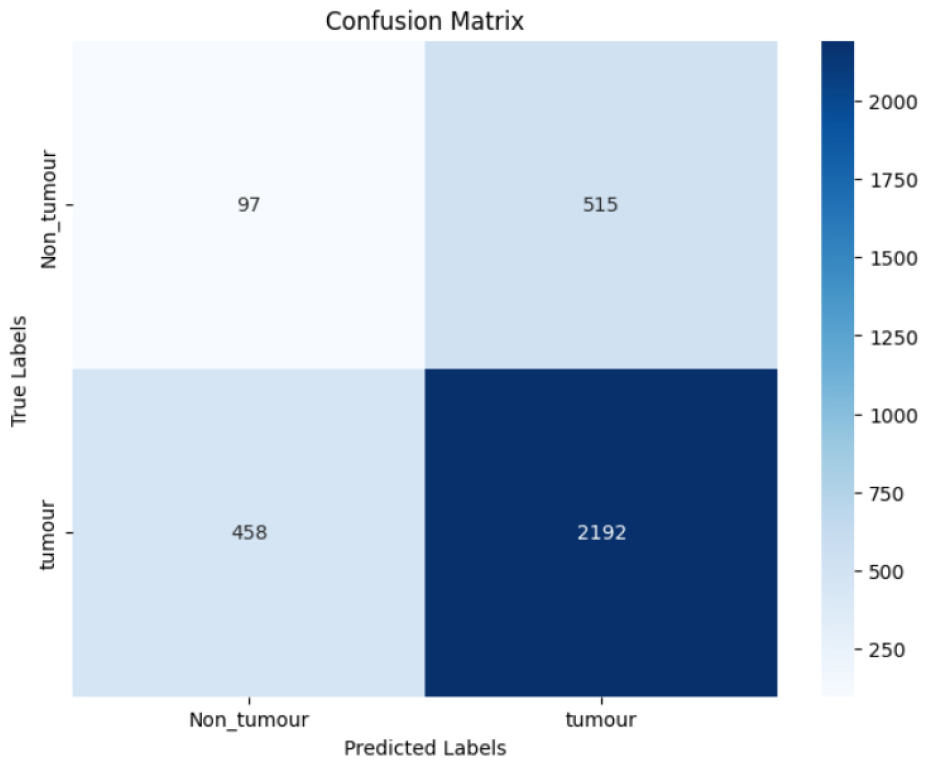
The confusion matrix in Figure 12 tells how well model classified data. 2192 tumor and 97 non-tumor cases were correctly identified. Nonetheless, it misclassified 458 tumor cases as non-cancers and 515 non-tumor cases as tumors. This suggests a class imbalance or model bias, as it achieves high tumor detection accuracy but makes significant errors in detecting non-tumor occurrences.
Results for VGG-19
VGG19 image classification uses the deep CNN structure that is recognized for its effectiveness and simplicity when dealing with challenging image recognition problems. Three fully connected layers, five max-pooling layers, and sixteen convolutional layers constitute the nineteen layers that comprise VGG19, culminating in a softmax for classification. It is an extension of VGG 16. VGG19 model uses 3x3 small filters in the network, enhancing model ability to learn complex features while maintaining controllable computational complexity. To implement VGG19, there is need to start by loading a pre-trained version of the model with weights trained using the ImageNet dataset, which is a potent feature extraction tool. The top (classification) layers are excluded, allowing customization for your specific dataset. Additional dense layers added on top of base architecture to accurately classifying between tumor and non-tumor images. With a training loss of 0.0220 and a validation loss of 0.0607, the VGG 19 model’s training accuracy was 0.9933.
Figure 13(a) illustrates the validation and training accuracy over 15 epochs. Despite the fact that these metrics settle between 96 and 98 percent of the time, initial oscillations and divergence point to overfitting or instability during training. As the parameters of model are adjusted, later epochs show convergence in training and validation accuracy, indicating higher generalization but with intermittent variance spikes.
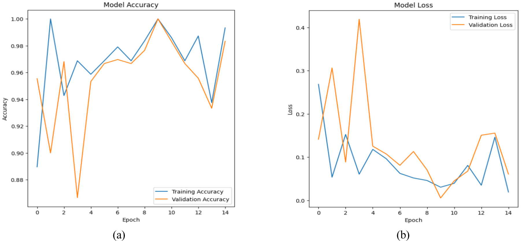
Figure 13(b) displays the validation and training loss patterns over the course of a model’s training phase epochs. The validation loss fluctuates a lot at first, but after a few epochs, it stabilizes and gets closer to the training loss. Reductions in training loss indicate learning, whereas changes in validation loss suggest either overfitting or noisy data.
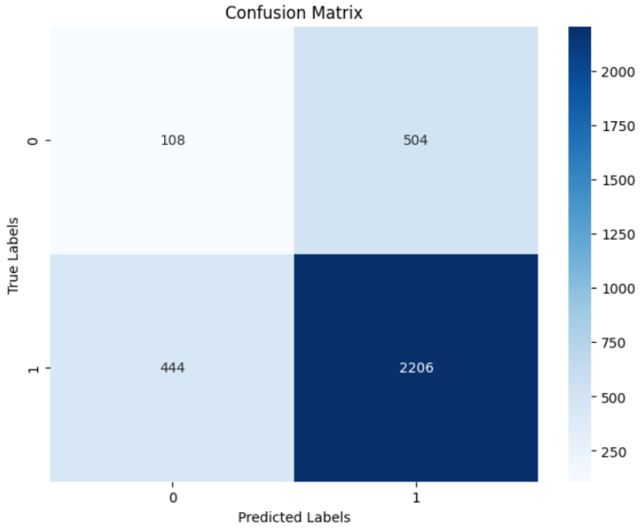
Figure 14 displays the classification performance of the model. It correctly predicts 108 true negatives and 2206 true positives. However, Model mislabelled 504 false positives (non tumor) and 444 false negatives (Tumor). The high rate of false positives and negatives suggests that there might be issues with the model’s balance or data distribution.
Results for EfficientNetB0
In order to optimize the trade-off between accuracy and processing economy, the EfficientNet family of models scales width, depth and resolution in a systematic and structured manner. These models have far fewer parameters and offer excellent accuracy when compared to traditional designs. Because users can select a model from versions ranging from EfficientNet-B0 to B7 that best meets demands from accuracy to performance, it is a flexible option for a different machine learning jobs. The training accuracy and validation accuracy of EfficientNetB0 were 0.9874 and 0.9817, respectively, with a training loss of 0.0359 and a validation loss of 0.1067.
Training and validation accuracy across ten epochs is explained in Figure 15(a). Accuracy is initially high throughout training and eventually stabilizes at nearly 100%. Validation accuracy has rapidly increased and is nearly equivalent to training accuracy by the third epoch. This implies that the model exhibits effective learning with minimal overfitting and generalizes effectively to new data.
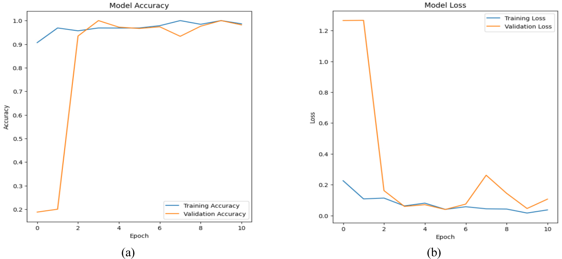
Figure 15(b) explain training and validation loss over 10 epochs. Both losses have significantly dropped by the second epoch, with the validation loss levelling off around the training loss. Effective learning and high generalization are demonstrated by the model’s ability to minimize overfitting while preserving low error rates on unseen data.
Figure 16 evaluate tumor classification model performance on true positive and false cases. 2210 were accurately identified tumors, or true positives. 102 genuine negatives, or correctly identified non-tumors, were found. There have been 510 false positives, or non-tumors that were mislabeled as tumors. There were 440 false negatives (tumor misidentified as non-neoplastic). The model detects malignancies more accurately than non-tumors.

Results for ResNet101
ResNet101, part of the ResNet (Residual Networks) family. It follows deep CNN architecture, intended to address challenges faces during training very deep networks. It has 101 layers and residual blocks, with shortcut connections in each block that divert one or more levels. It helps mitigating vanishing gradient problem, helps in train deep networks and achieve high performance on classification tasks. ResNet101 excels in medical image detection and classification, providing a strong balance between depth and computational cost. Training accuracy of ResNet101 model was 0.9994 with training loss of 0.0017 and validation accuracy was 0.9904 with validation loss of 0.0611.
The accuracy of training and validation throughout 25 epochs is shown in Figure 17(a). Following epoch 5, training accuracy stays constant at about 1.0, but validation accuracy rapidly increases and stabilizes. The close alignment of the two indicates robust model generalization with little overfitting to the training set.
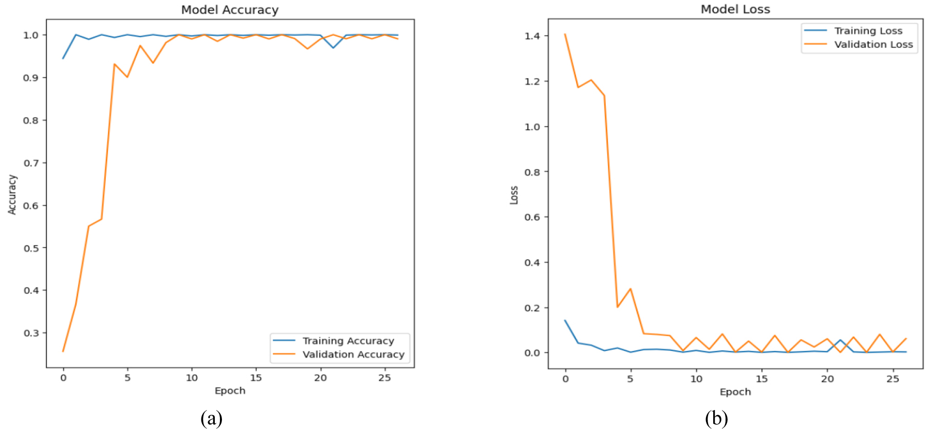
Figure 17(b) explains training and validation loss over 25 epochs. Training loss gradually decreases until it reaches zero. Validation loss has significantly reduced by epoch 5 and remains low with just minor fluctuations. The close alignment of both losses indicates a well-generalized model with minimal overfitting and effective learning.
Figure 18 shows prediction of “tumor” with more accuracy (2651 true positives) than “non_tumor” (586 true negatives). It had 0 false negatives and 25 false positives, indicating intermediate misclassification rates. Despite favouring tumor identification, the model’s non-tumor prediction has to be enhanced.

This study presents an inclusive evaluation of tumor classification. First assessed the impact of datasets on classification, on publicly approved datasets used in the model development. Due to the differences in size distribution and output classifications among datasets (a, b, c and d), the outcomes were highly inconsistent. However, the recommended method produced some promising results, with ResNet101 showing the best accuracy at 99.94%.
Comparing the success of DL models for brain tumors classification reveals varying degrees of accuracy. The reliability of the VGG architecture in medical imaging tasks was demonstrated by VGG-16 and VGG-19, which ranked second and third, respectively, with an impressive accuracy of 99.36%. EfficientNetB0 performed somewhat worse, demonstrating efficiency but a little less precision in this scenario with an accuracy of 98.74%. ResNet101 was the most accurate model, demonstrating its mastery of deep feature extraction and complex data representation with an impressive 99.94% accuracy rate. These results show that ResNet101 dominates tasks that demand high accuracy for brain tumor classification.
A deep CNN architecture called ResNet101, which is a member of the Residual Networks (ResNet) family, was created to tackle the problem of training extremely deep networks. ResNet is fine-tuned and trained to identify tumor regions from MRI scans. Masked images, which highlight the tumor and eliminate irrelevant details, are produced from this step. The workflow ensures better data inputs for classification and analysis by segmenting the images followed by leverage Fine tune ResNet101 for detecting brain tumor with higher accuracy. The ResNet101 model is a deep CNN architecture that can learn intricate characteristics that are helpful for categorizing pictures of brain tumors because it was pre-trained on big medical dataset followed by augmented with tumor dataset along with segmentation for higher accuracy. Table 2 explains comprehensive evaluation metrics for tumor and non-tumor classification.
Table 2.
Evaluation metrics for tumor and non-tumor classification
| Class | Model accuracy | TP | TN | FP | FN | Accuracy | Precision | Recall | F1 Score |
| Tumor | 99.94% | 2651 | 586 | 25 | 0 | 0.9679 | 0.9635 | 0.9985 | 0.9979 |
| Non Tumor | 586 | 2651 | 0 | 25 | 0.9980 | 0.9930 | 0.9960 | 0.9952 |
The proposed model outperforms with an overall accuracy of 99.94%. For the Tumor class, it has a high recall (0.9985) and F1-score (0.9979), indicating a high sensitivity. Similarly, the non-tumor class has a high precision (0.9930) and F1-score (0.9952), demonstrating the model’s robustness and reliability in binary classification. VGG 16, VGG 19, ResNet101, EfficientNetB0 were chosen because of their demonstrated efficacy in medical imaging for detecting Brain tumor. These designs provide deep feature extraction, robust gradient flow, and hybrid strengths, which improve accuracy, minimize overfitting, and improve model generalization in brain tumor detection by leveraging superior convolutional and residual learning capabilities. VGG 16 is a deep CNN architecture that can learn intricate characteristics that are helpful for categorizing pictures of brain tumors because it was trained on a combined dataset following segmentation. The EfficientNetB0 family of models scales depth, breadth, and resolution in a systematic manner to maximize the trade-off between accuracy and processing economy.
Table 2 displays the comparison of various DL architecture used for binary tumor detection either tumor or no tumor. The proposed model shows the highest accuracy of 99.94% over state-of-the-art advance DL architectures.
Table 3 displays the comparison of various deep learning architecture used for binary tumor detection either tumor or no tumor. Proposed model shows the highest accuracy of 99.94% over state-of-the-art advance DL architectures.
Conclusion and Future Scope
Early detection may be crucial to preserving lives because brain tumors have the potential to be deadly or seriously damaged. This work proposes robust categorization method for an instant, precise, and early diagnosis to prevent dreadful effects. Brain MRIs were divided into two groups using a deep CNN-based architecture: tumor and no tumor. The categorization model was developed and evaluated on merged & combined dataset. Furthermore, the proposed model outperformed models and state-of-the-art publications. ResNet101 outperformed the others, followed by VGG-16 with 99.36% with an accuracy of 99.94%, VGG-19 with 99.33%, and EfficientNetB0 with 98.74%. However, if additional real-world MRI data for the model’s segmentation and training is available, then ResNet101 model might be more helpful. This research also highlights sustainable methods in medical imaging by utilizing transfer learning methods to enhance model efficiency and minimize computational expense.
Future research will concentrate on improving the generalization of the model using more varied real-world MRI data for better segmentation and training. The model can be expanded in the future to incorporate multi-modal imaging data, including PET and CT scans, and to account for additional types of brain illnesses. As an aspect of future work, it is possible to consider Explainable Artificial Intelligence (XAI), with the frameworks like LIME and Grad- CAM being used to clarify the model purpose and logic. In addition, these innovations have the potential for urban health use, providing scalable AI-based diagnostic solutions for various healthcare infrastructures. Furthermore, investigating transfer learning, hybrid architectures, and sophisticated data augmentation methods may improve the system’s accuracy and resilience, enabling prompt intervention and early detection for the diagnosis of brain tumors in various populations.
