

Introduction
Data
Passenger trajectory data acquisition
Data labeling
Feature Extraction
Methodology
Selection and Optimization of Base Classifier
Ensemble for model combination
Passenger Mobility Index (PMI)
Analysis
Classification results
Evaluation of Passenger Mobility Performance
Conclusion
Introduction
Urban railways have high frequencies compared to other public transportation systems and provide the convenience of connection between transportations; however, there is severe congestion during rush hours. As congestion at the station has increased, it is necessary to improve pedestrian space [1]. For this, significant effort has been invested in several countries to evaluate the pedestrian level of service (LOS) [2, 3, 4]. According to the Highway Capacity Manual by the Transportation Research Board [5], the pedestrian flow rate, which incorporates pedestrian speed, density, and volume, is a measure for evaluating pedestrian LOS. However, the pedestrian LOS is investigated for 15-min intervals on a specific day or time, and therefore, there is a limitation in evaluating the pedestrian space in subway stations in real-time. Thus, the monitoring of passenger mobility in real-time is necessary to evaluate pedestrian space and route information systems within the smart city based on sustainable facilities and artificial intelligence technology.
“An image detection system such as CCTV can be used to monitor the pedestrian space environment, but it is inefficient in that video data cannot provide valid information when the lighting in spaces is dark [6]. In addition, to detect wandering pedestrians using the image detection systems, it is difficult to monitor continuously track the trajectory of individual pedestrians and determine roaming behavior.” “A Light Detection And Ranging (LiDAR) sensor, which has been recently used in the driving environment recognition technology for autonomous vehicle systems, is used to detect and track objects with a wide detection range and high accuracy [7, 8].” When a detection area between the sensors overlaps partially, individual passengers can be tracked continuously. Therefore, it is possible to monitor and evaluate the pedestrian space in subway station by using the pedestrian trajectory data collected based on the LiDAR sensor. Further, this data can be used to analyze the passenger trajectory patterns in the subway station by extracting individual passenger trajectories. The passenger trajectory data, which includes the two-axis coordinates, speed, acceleration, and direction angle of an individual passenger, are useful for detecting abnormal trajectory patterns that are ineffective movements between the start and endpoint [9].
The evaluation of passenger mobility in the public transport facility including subway stations is a backbone of developing various measures to enhance the quality of public transportation services, which motivates our study. This study developed a methodology for identifying abnormal passenger walking patterns, which supports the evaluation of passenger mobility performance, based on the analysis of individual trajectories data obtained from LiDAR sensors. Abnormal passengers were classified using an ensemble method, a combination of several base classifiers, to achieve high accuracy. The classification procedure for passenger trajectory patterns comprises four steps. First, field data preparations were conducted to collect passenger trajectory data for morning peak, afternoon nonpeak, and afternoon peak hours at the Samsung station in Seoul, Korea. Further, this step included labeling passenger trajectories using feature vectors that were extracted toward the reliable characterization of passenger walking trajectories. Second, the decision tree (DT), support vector machine (SVM), and artificial neural network (ANN) were selected as the base classifiers and optimized. Next, the ensemble method of combining three base classifiers was applied and the characteristics of the abnormal passenger trajectories were presented. Finally, this study further devised a performance measure to identify the performance of passenger mobility in subway stations, referred to as passenger mobility index (PMI), based on the classification results.
The remainder of this report is organized as follows. In section 2, the passenger trajectory and labeling data for the Samsung station are described. Section 3 introduces an overall framework for the proposed methodology, including optimization techniques for base classifiers and ensemble methods using weighted majority voting. Section 4 presents the results of the analysis. Finally, Section 5 presents the conclusions, summarizes the results, and discusses future research.
Data
Passenger trajectory data acquisition
Recently, advanced sensor and communication technologies have been widely applied to provide various services for transportation users and operators. In particular, the LiDAR sensor, which has been widely used as a key component of autonomous vehicles, is easy to install and expand, with a fast data acquisition process. Consisting of a transmitter and a receiver, a LiDAR sensor detects the distance, direction, and speed from the object by calculating the duration of the returning short light pulse laser. The sensor has an excellent range and spatial resolution in weather conditions of various lighting and temperatures. “The LiDAR sensor has the advantage to precisely track objects and process data quickly, enabling it to smoothly track a passenger’s movement, even in a complex room such as a subway station.” More technical details of the LiDAR sensor can be found in the referenced literature [10].
This study used a commercialized pedestrian trajectory collection system (PTCS) developed by LG Hitachi, which is based on a 2D-LiDAR sensor, to collect individual pedestrian trajectory data in a public facility. The PTCS affords customized communication, with the maximum sensing range of a LiDAR sensor approximately 15 m and 270°, with a 5-Hz band. Continuous passenger trajectories can be collected by overlapping the detection areas between LiDAR sensors. Collected and recorded every 0.2 s on a server computer connected to the sensors, the passenger trajectory data include the two-axis coordinates, walking speed, and the direction angle. Based on tracking results, the PTCS also provides visualization solutions, such as real-time pedestrian tracking systems and a heat-map. Further information regarding the PTCS can be found in the referenced literature [11].
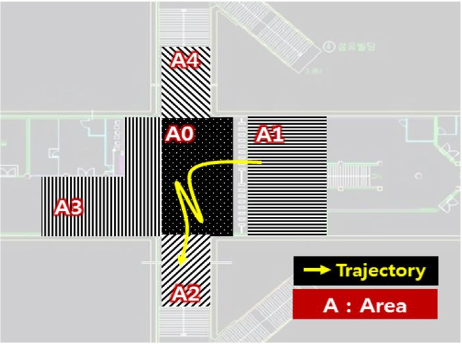
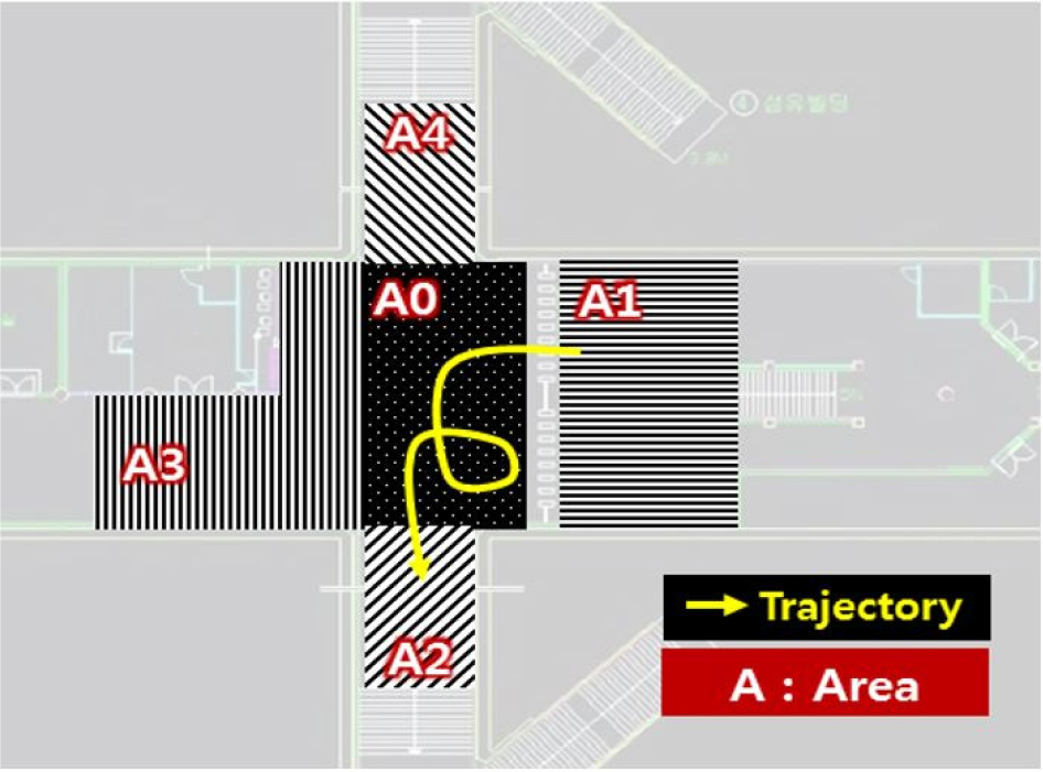
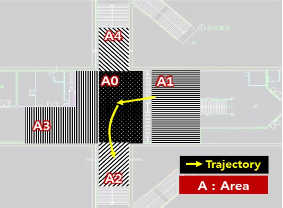
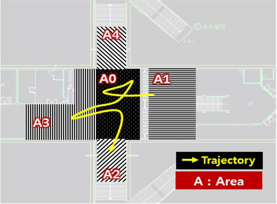
The passenger trajectory data was collected by the PTCS near the passage from the ticket gate to exit 3-6 at the Samsung station, which is one of most crowded subway station in Korea, as shown in Figure 1. “The un-continuous and incomplete trajectories were extracted based on the start and endpoint of individual pedestrian trajectory and removed as outliers. When the start and endpoints are A1 to A4, it is assumed that they have to pass through A0, which is defined as the waiting area (shown in Table 1). If the start and endpoint of the trajectory were A0, it was determined to outliers because it was not possible to know which direction it came and went. Also, during the movement from the start to endpoint, the pedestrian trajectory that did not include A0 and had the same start and endpoint represented as an interrupted trajectory. The unknown trajectory patterns were excluded from this study.” A total of 15,247 passenger trajectories collected during three time periods, which include morning peak hours, afternoon nonpeak hours, and afternoon peak hours, were used in the analysis of this study.
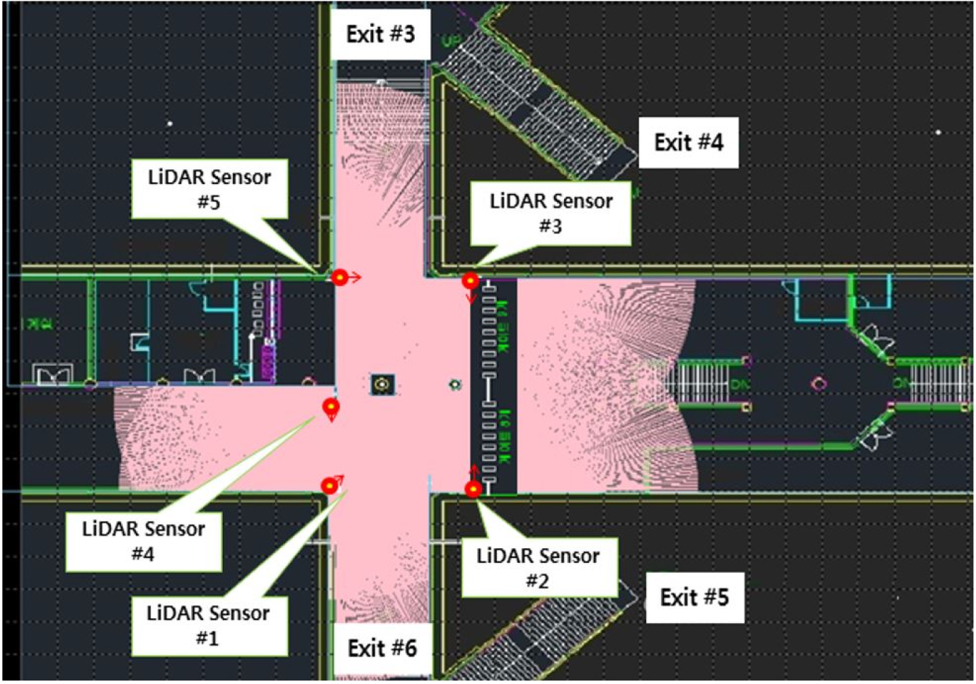
Table 1.
Definition of abnormal passenger trajectory patterns
Data labeling
Indoor travel patterns were referred to as roaming, and they were classified as random, pacing, and lapping; random implies a roundabout or haphazard travel to many locations within an area without repetition; pacing is a repetitive back-and-forth movement within a limited area; and lapping involves repetitive travel characterized by large circular areas [12]. Jo et al. distinguished three types of abnormal trajectory patterns as pacing & lapping, stay, and inefficiency when a spatial range is specified as pedestrian space in a subway station [9]. The type of pacing & lapping refers to the repetitive movement within a limited area, and the type of stay indicates the act of staying at specific point for a long time. Further, the type of inefficiency is defined as unpredictable movement while passengers move from the start to the endpoint. Table 1 summarizes the abnormal passenger trajectory patterns. For any of the three types of roaming, the individuals were classified as abnormal passengers and labeled as “1”; otherwise, they were classified as normal passengers and labeled as “0”. The labeling results classified 1,249,300, and 1,731 passengers as abnormal passengers in the morning peak, afternoon nonpeak, and afternoon peak hours, respectively.
Feature Extraction
Seven feature vectors were derived to characterize the individual passenger walking trajectories to classify abnormal passengers. Each feature vector was calculated based on the cells in the passenger monitoring space while moving from the start to the endpoint, and the size of the cells was set to 400 × 400 () considering the average shoulder width of adults in Korea [13]. Accordingly, coordinates of the passenger trajectory data and cells were matched to determine whether the passenger returns to the same space or if they stay in a cell for a long time. “Derived feature vectors are as follows [9]:”
•: Number of cells
•: Number of occupations for a certain cell
•: Standard deviation of walking speed
•: Standard deviation of direction angle
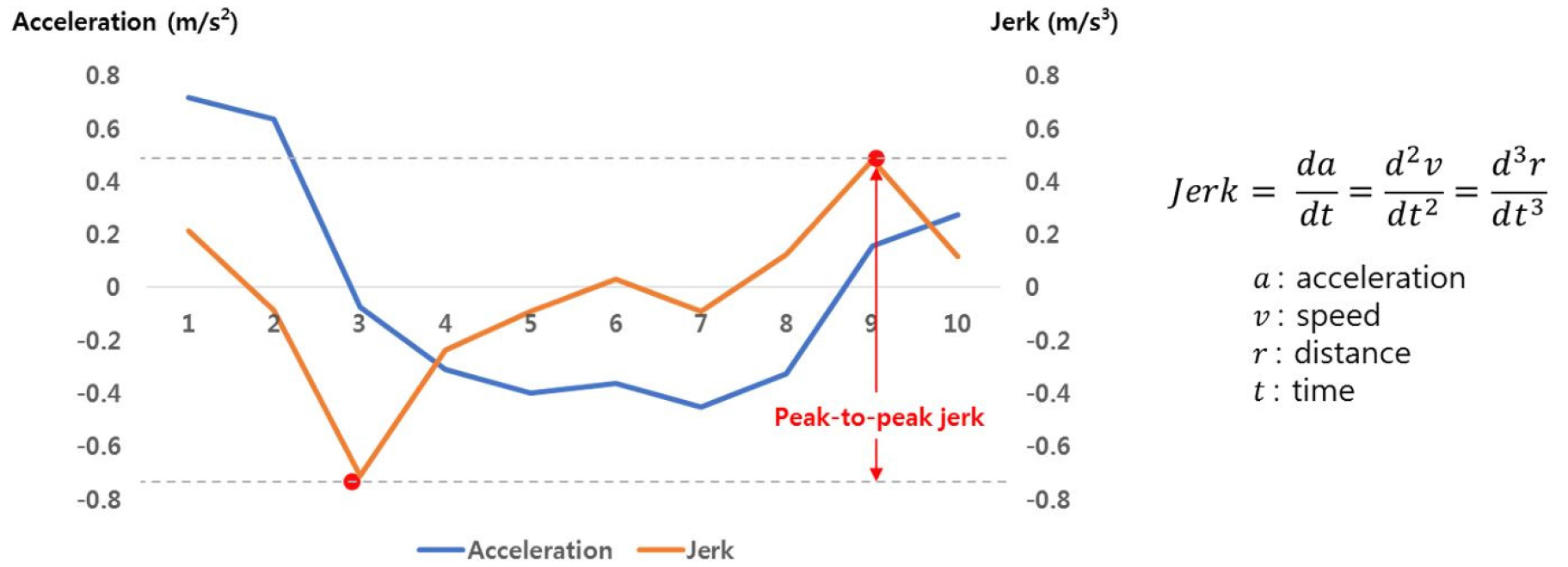
•: Peak-to-peak jerk representing the difference between maximum and minimum value of jerk as shown in Figure 2. “The jerk is a measure that evaluates driver comfort and driving stability as the rate of change in acceleration profiles, which increasing jerk means that the stability decreases [14]. This study used the jerk as an indicator of the walking stability of pedestrians in the subway station.”
•: Average duration for occupation
•: Maximum duration for occupation
Methodology
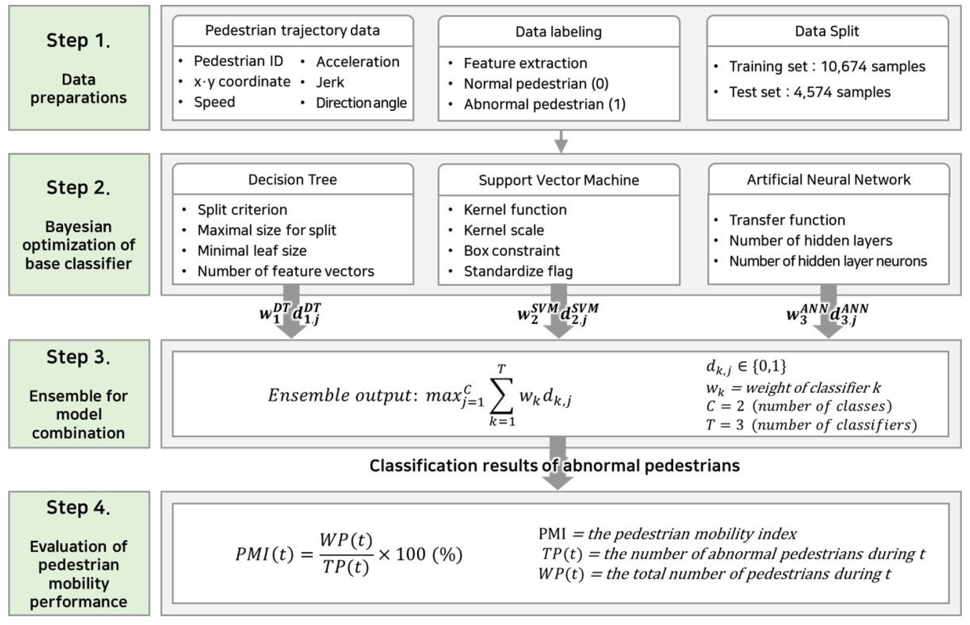
This study developed a methodology to detect and classify passengers with abnormal trajectory patterns using individual passenger trajectory data collected through LiDAR sensors. An overview of the methodology is presented in Figure 3. The first step is data preparation, which includes data collection, feature vector extraction, and labeling. Feature vectors that characterize the passenger walking trajectories were derived and used to label normal/abnormal passengers [9]. The labeled data were divided into the training set and test set by 70% and 30%, respectively. The second step is performing Bayesian optimization on the base classifier. The base model for the passenger trajectory classification was selected as the decision tree (DT), support vector machine (SVM), and artificial neural network (ANN). Further, the optimal hyperparameters of each base classifier that minimize the correct classification rate (CCR) were derived. In the third step, the results derived from the base classifiers were integrated by applying weighted majority voting for the ensemble methods, and the abnormal passengers were identified. Next, the performance of the classifiers was evaluated using the confusion matrix. Once a classification tool to identify passenger trajectory patterns is developed, the final step of the proposed methodology in this study is to devise a performance measure to identify the performance of passenger mobility in subway stations, referred to as passenger mobility index (PMI), based on the classification results.
Selection and Optimization of Base Classifier
An important process to detect abnormal passenger using walking trajectory data is to select the appropriate classifier. To improve the performance of the classifiers, it is necessary to adjust the classifier’s hyperparameter before the start of the learning process. Decision tree [15], support vector machine [16], and artificial neural network [17] are well known supervised learning models for classification analysis. “Machine learning techniques have applied to data mining of moving object trajectories to classify patterns including spatiotemporal factors [18, 19, 20].” In this study, these classifiers are selected as the base model of the ensemble method, and they are performed to determine abnormal trajectory patterns.
Decision tree
A decision tree (DT), which is a method commonly used in data mining, can be used for classification or regression for decision making [15]. The DT model has a decision flow chart structure for testing attributes for each node, and therefore, process can be easily understood and explained. Algorithms for constructing DTs usually work top-down, by choosing a variable at each node that best splits a given set of data into criteria. “In general, these criteria are usually used to measure the homogeneity of the target variables within the subsets [15].” Therefore, DTs have different models according to the split criterion of each node, and nodes and branches are divided into different algorithms through pruning. “In addition, a DT classifier requires parameter tuning as listed in Table 2; the pruning parameter is optimized to avoid overfitting [15, 21].”
Table 2.
Hyperparameter for decision tree
| Hyperparameter | Description | Reference | |
| Split criterion | Information gain | The concept of entropy and information content from information theory | [15, 21] |
| Gini impurity | A measure of how often a randomly chosen element from the set would be incorrectly labeled if it was randomly labeled according to the distribution of labels in the subset | ||
| Variance reduction | The total reduction of variance that occurs during node split | ||
| Maximum size for split | Maximal number of decision splits or branch nodes | ||
| Minimum leaf size | Minimum number of leaf node observations | ||
| Number of feature vector | Number of predictors to select at random for each split | ||
Support vector machine
The support vector machine (SVM) determines a hyperplane that has the largest distance to the nearest training data point of any class called the margin. The SVM model sets a boundary around the area where points belonging to the same class are gathered. The decision boundary of N samples with training data and target variable is expressed as (1)[22]:
where is a normal vector representing the weight of a decision hyperplane and the is a bias. The hyperplane separates the feature space into two regions, > 0 and < 0. The distance from any point to the hyperplane is equal to (2)[22]:
where is the distance from a support vector to the hyperplane . The conditional optimization problem to maximize , which is the margin of the support vectors of the two classes, can be represented by a minimization problem as (3)[22]:
where is any point on or below the boundary belongs to another class, with label 1 or -1. If it is not possible to divide the two classes into a linear hyperplane, we use a kernel function that converts the linearity into a nonlinear space. In general, Gaussian radial basis function, polynomial kernel function, and linear kernel function are represented as (4)[23]:
The SVM models determine different hyperplanes according to the kernel functions, and the performance of the model depends on parameters such as the kernel scale; the parameters were optimized to improve classification accuracy. “Table 3 summarizes the hyperparameters for SVM [16, 23].”
Table 3.
Hyperparameter for support vector machine
| Hyperparameter | Description | Reference | |
| Kernel function | Gaussian of RBF | Gaussian or Radial Basis Function kernel, default for one-class learning | [16, 23] |
| Linear | Linear kernel, default for two-class learning | ||
| Polynomial | Polynomial kernel of order q | ||
| Kernel scale | Utilized to calculate a matrix applying the appropriate kernel norm by dividing all the elements of the feature vector x to the kernel scale | ||
| Box constraint | Adjust the boundary of data (number of support vector) | ||
| Standardize flag | Standardization of feature vector to apply to the classifier | ||
“Piciarelli et al. [24] collected video data to track the trajectories and applied the SVM to identify anomalous trajectories. The previous study has been shown excellent performance in detecting exceptional patterns from typical patterns. Sun and Ban [25] collected the vehicle trajectory data using GPS data. SVM method have applied to binary-class classification, which misclassification rates of the training set and the test set were derived as 1.6% and 4.2%, respectively.”
Artificial neural network
The artificial neural network (ANN) is a computing technique that is inspired by biological neural networks constituting the human brain. The ANN model is composed of an input layer that accepts input data, hidden layers that compute the result of processing input values, and an output layer [26]. Each layer consists of nodes and the results are derived by the interaction of nodes and the transfer functions. The output of the node depends on the transfer functions typically used as step, sigmoid, hyperbolic tangent, linear, and softmax functions represented as (5):
The ANN model is divided into two stages: i) feed-forward, in which the signal is forward transmitted only by allowing connections between layers, and ii) back-propagation, in which the output values calculated from the model and the error with the actual value is estimated and propagated in the opposite direction. The pattern recognition networks applied in this study are feedforward networks that can be trained to classify inputs according to target classes. Therefore, the “ANN has different models according to network architecture specifications such as the number of hidden layers and hidden nodes; the hyperparameters as listed in Table 4; they were optimized to minimize the error [17, 27].”
Table 4.
Hyperparameter for artificial neural network
| Hyperparameter | Description | Reference | |
| Transfer function | Step | A finite linear combination of indicator functions of intervals | [17, 27] |
| Sigmoid | The input and squashes the output into the range 0 to 1 | ||
| Hyperbolic tangent | Related to a bipolar sigmoid which has an output in the range of -1 to 1 | ||
| Linear | Linear transfer function | ||
| Softmax | To map the non-normalized output to a probability distribution over predicted output classes | ||
| Number of hidden layers | The number of hidden layers | ||
| Number of neurons | The number of neurons in the hidden layers | ||
“Zhao et al. [28] tried to distinguish pedestrians and vehicles based on a neural network by installing a LiDAR sensor on the roadside. The classification accuracy of the developed model was found to be over 93%. In addition, ANN classified pedestrians and vehicles within the detection range of the LiDAR sensor [29]. As a result, accuracy of model was 96.5%, indicating excellent performance.”
Bayesian optimization
Bayesian optimization outperforms other state-of-the-art global optimization algorithms [30] and is applied for tuning model hyperparameters [31]. The objective function of the Bayesian optimization strategy is maximized to find set represented by (6):
where in this study represents the correct classification rate (CCR) of the models, and is derived to optimize the hyperparameters that maximize CCR. Bayesian optimization constructs a probabilistic model for , and the process can be outlined as follows: i) is assumed to follow the gaussian process (GP) prior. Then, the model is learned using the given data D = ; ii) Calculate the acquisition function for data not included in D; iii) Include the data point with the largest acquisition function value in D. The acquisition function is a measure for finding hyperparameters that affect the global optimum so that the maximum CCR can be obtained. The types of acquisition function are expected improvement (EI), probability of improvement (PI), and upper confidence bound (UCB). The EI is generally known to minimize the errors of the predicted [32] and is defined by (7)[30]:
where , , and represent the maximum, average, and standard deviation of CCR predicted for hyperparameters, respectively. Furthermore, is the normal cumulative distribution function, and is the probability density function for . To calculate the average and standard deviations of prediction by using GP, which is a suitable model for Bayesian optimization algorithms, because of incremental learning and variance computation easily [33, 34].
Ensemble for model combination
The concept of an ensemble is a multiple classifier systems (MCS) that integrated the outputs of several classifiers. “The ensemble method, which can convert weak learners to strong learners, constructs an optimal model by combining several classifiers by using a given data set. Generally, the outputs are obtained by voting to combine the results of the base model [35, 36].” “In pattern recognition, it has been reported that the performance of the ensembles is better than obtained by any of the constituent learning algorithms alone [37, 38].” “The ensemble method that combines multiple classifiers improved classification performance, model prediction, generalizability, and robustness [39]. Hernandez et al. [40] proposed an MCS to classify 54 vehicle types by collecting data from a weigh-in-motion (WIM) system and inductive loop detectors (ILD). The proposed MCS is a classifier that combines naive bayes classifier, DT, SVM, multi-layer feedforward neural network, and probabilistic neural network. Bejani and Ghatee [41] integrated four machine learning algorithms including DT, SVM, K-Nearest Neighbor, and multi-layer perceptron into a voting method to classify congested and normal traffic conditions. The performance improved when each prediction results are combined.” The voting and non-voting methods are used for combining classifiers. The most common method is uniform voting, which is used when outputs are obtained by applying the same weight to all the base models. Another common method is weight voting, in which the weight is proportional to the CCR of each base classifier, as represented by (8)[42]:
The decision of the classifier is denoted as , and , where K is the number of classifiers and C is the number of classes. If the classifier chooses class j, then =1; otherwise, it is 0. Furthermore, weights can be normalized so that they add up to 1 for easier interpretation.
Passenger Mobility Index (PMI)
The PMI has potential for use in evaluating walking spaces in subway stations. PMI is defined as the percentage of the total number of passengers to the number of abnormal passengers, and it can determine analysis periods based on the purpose of analysis and utilization. PMI is represented by (9):
where PMI(t) is the passenger mobility index, TP(t) is the total number of passengers, and WP(t) is the number of abnormal passengers during t. PMI varies from 0 to 100. When PMI is zero, there is no abnormal passenger. On the other hand, if PMI is 100, all passengers are wandering, indicating that there is severe congestion in subway station.
Analysis
Classification results
This study developed an ensemble model combining DT, SVM, and ANN to classify normal and abnormal passengers in a subway station. A total of 15,247 data samples of 11,967 (78.5%) normal passengers and 3,280 (21.5%) abnormal passengers were used for the analysis. The number of data samples in the training set and test set of each base classifier was divided into 10,673 (70%) and 4,574 (30%), respectively. The seven feature vectors that can show the characteristics of passenger trajectories were set as input data. The class label for normal passengers was set as 0 and that for abnormal passengers was set as 1, and these were used as target variables. The optimal set of hyperparameters for each classifier trained using the training set is listed in Table 5. In addition, the confusion matrix applying the test data to the optimized base classifiers and ensemble model through the training data are summarized in Table 6.
Table 5.
Results of optimal hyperparameters by base classifier
Table 6.
Confusion matrix for base classifiers and ensemble
The most commonly used performance measure for model evaluation is accuracy, which is a measure of how closely the predicted value of the model is equal to the true value. In addition, sensitivity, specificity, and precision are used for model evaluation. Sensitivity and specificity are measures of the ability to classify normal passengers as normal and abnormal passengers as abnormal, respectively. Precision is a measure of the ability of a researcher to classify data of interest [43]. The accuracy of the ensemble model was 94.4%, which has the highest accuracy compared with that of the other base model. The sensitivity when classifying normal passengers as normal was estimated to be 96.7% for the decision tree and ensemble method. In addition, the specificity for abnormal passengers was 86.4% for the ensemble method, which is approximately 18% higher than that of the ANN model. Finally, the precision was 96.3% for the ensemble method, which is higher than that of each base classifier. The results of the comparison of performance measures for each classifier are summarized in Table 7.
Table 7.
Comparison of performance measures
Evaluation of Passenger Mobility Performance
PMI varies from 0 to 100. When PMI is zero, there is no abnormal passenger. On the other hand, if PMI is 100, all passengers are wandering, indicating that there is severe congestion in subway station. As a result of classifying the passengers by applying the ensemble method, 970 abnormal passengers could be identified out of 4,574 passengers. Therefore, the PMI of the Samsung station was calculated to be 21.2%. If the additional passenger trajectory data can be collected in the future, it is important to establish an appropriate analysis period for monitoring a subway station. In addition, it is possible to select the target subway station that needs improvement in the walking space by deriving PMIs for various subway stations.
As an exemplar application of the mobility performance analysis, the mobility of passengers moving from the ticket gate (A1) to three exits (A2, A3, and A4) was compared using the proposed PMI obtained during the morning peak hours, 7 a.m. to 9 a.m. Table 8 presents the result of identifying abnormal passenger trajectories with three routes (Route 1, Route 2, and Route 3) from the ticket gate and each exit. 336 passengers out of 2,706 passengers who exited using Route 2 were found to be abnormal, and a PMI of 12.4% were then observed. Meanwhile, 72.4% and 14.8% of PMI were observed in Route 3 and Route 4, respectively. Therefore, it can be said that Route 3 needs to be improved in terms of the passenger mobility performance.
Table 8.
Route definition and PMIs
| Route | The number of passengers | The number of abnormal passengers | PMI | 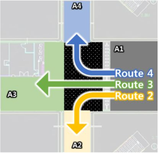 |
| Route 2 | 2,706 | 336 | 12.4% | |
| Route 3 | 174 | 126 | 72.4% | |
| Route 4 | 2,706 | 401 | 14.8% |
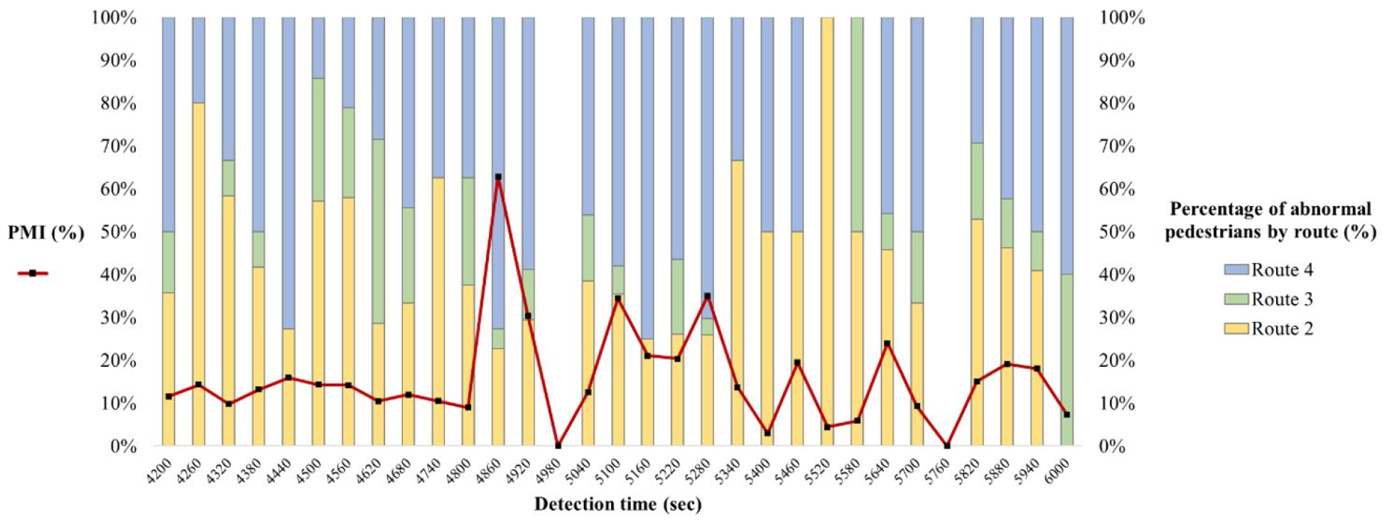
The proposed methodology also allows for real-time monitoring of passenger mobility. For example, Figure 4 illustrates a temporal pattern of PMIs observed for each route during 30 minutes when the analysis time period is set to 60 seconds. A relatively high PMI indicates that the passenger mobility performance becomes worse, which requires the implementation of appropriate improvement measures.
Conclusion
Increase in congestion has necessitated improvements of pedestrian space environments in subway stations. Various studies have suggested measures for evaluating the pedestrian level of service. However, there is a limit to evaluate pedestrian space in real-time, as pedestrian LOS is investigated at a specific day or time. Recent advances in sensor and communication technology have provided opportunities to collect various data in real-time. It is possible to detect abnormal passenger as well as evaluate walking space by using LiDAR sensors capable of tracking individual passengers continuously. It is an essential requirement for monitoring pedestrian space in a subway station, that is, providing route information to minimize roaming passengers and extracting them from a security perspective. Therefore, in this study, a methodology was developed to identify and classify passengers that show abnormal trajectory patterns based on LiDAR sensors in a Samsung station.
Feature vectors were extracted for reliable characterization of passenger walking trajectories. The classification of abnormal passenger trajectory patterns is based on an ensemble method combining several classifiers, which include DT, SVM, and ANN as base models. The accuracy of the ensemble model was 94.4%, which is higher than that of each base classifier. The sensitivity, specificity, and precision were also derived from the highest ensemble model. It is important to develop a model with high specificity in the classification of abnormal passengers in a subway station, and a model with few false positives (FPs) should be selected. This is because it is more critical to judge abnormal passengers as normal rather than normal passengers as abnormal. The specificity of the ensemble model was the highest at 86.4%, and the FP was the least at 134, which is better than that when a classifier was applied alone. The model proposed in this study can monitor and evaluate the passenger mobility in a subway station through the detection of walkers. Furthermore, it is expected that passengers who show abnormal trajectory patterns will be paid more attention to identify the cause of wandering. Finally, this study further devised a performance measure to identify the performance of passenger mobility in subway stations based on the classification results. The PMI analyses were presented as examples of applying the proposed methodology in monitoring the passenger mobility.
Although important issues were identified by this study, additional research should be conducted. First, this study was conducted using a limited passenger trajectory data set. Therefore, by constructing a sensor-based database is constructed in a subway station and collecting passenger trajectory big data, it is possible to obtain more reliable and realistic results. Second, to verify the results, it is necessary to compare passenger characteristics by matching the passenger trajectory data and the collected video data at the same time. In future research, a methodology for video-based passenger tracking should be developed. Third, this study selected three base classifiers, but an ensemble algorithm including another classifier such as the K-nearest neighbor, Naïve bayes, and probabilistic neural network should be developed. Because each classifier derives different prediction results, it is expected that the performance of the ensemble model combining various classifiers will increase. “Finally, to increase the reliability of the proposed methodology, it is necessary to classify wandering pedestrians and analyze walking patterns by collecting pedestrian trajectories for various space types such as 3-way and 5-way intersection.” “In addition, there is a need for a study to analyze walking characteristics by time of day morning peak, afternoon nonpeak, and afternoon peak. The proposed methodology will be advanced by extracting features reflecting different walking characteristics for each time period.”
An effort will be needed to systematically analyze and to derive practically applicable results for future research. The passenger mobility evaluation technology, which provides sustainable services based on smart facilities, can detect roaming passengers and identify the cause of wandering by paying more attention to abnormal passengers. In addition, it is possible to suggest a countermeasure such as improvement of walking facilities and route information system by monitoring.
