

Introduction
Material and Methodology
Dataset
Data Preprocessing
Deep Learning model
SHAP Analysis
Model Evaluation Metrics
Result and Discussions
Conclusions
Introduction
The United Nations Sustainable Development Goals (SDGs) —particularly Goal 7 on Affordable and Clean Energy, Goal 12 on Responsible Consumption and Production, and Goal 13 on Climate Action— highlight the vital role of sustainable energy management in addressing global climate challenges [1]. As a critical natural resource, energy profoundly affects climate change. Therefore, promoting its sustainable use and reducing carbon dioxide (CO2) emissions are essential steps toward mitigating global warming [2]. Rising atmospheric CO2 levels, largely driven by human activity, pose serious threats to ecosystems, public health, and the planet’s long-term livability [3].
The 2021 Global Carbon Budget reports that approximately one-third of all CO2 emissions over the past 70 years occurred after 2000 [4], with fossil fuel combustion identified as the primary contributor. This surge in emissions is a key factor behind the ongoing rise in global temperatures [3]. Since the adoption of the Paris Agreement in 2015—which aims to limit warming to well below 2°C, preferably 1.5°C, above pre-industrial levels—nations have introduced policies to curb emissions. However, global emissions continue to rise, underscoring the urgent need for more robust and coordinated action [5]. The heat-trapping nature of CO2 amplifies the greenhouse effect, accelerating temperature increases. Currently, China, the United States, the European Union and the United Kingdom, and India are the world’s largest CO2 emitters [6].
The residential sector plays a significant role in global greenhouse gas (GHG) emissions, accounting for more than 60% of total emissions through its consumption of goods and services [7]. Regional disparities are evident: residential CO2 emissions account for about 20% in the U.S. [8], 30–40% in China, and 44% in Canada [9]. In Japan, the residential sector accounted for approximately 40% of national emissions in 2018; however, direct CO2 emissions from this sector were only 4.84% [10]. These figures illustrate the critical need to address household consumption patterns in pursuit of climate targets [11].
In the U.S., homes have an average lifespan of around 40 years, posing a challenge to rapid decarbonization. Key construction decisions—such as building size, heating systems, materials, and housing type—significantly impact long-term emissions. Post-World War II suburban development policies led to widespread sprawl, resulting in per capita energy use and emissions far exceeding global norms. Without immediate interventions, these homes risk contributing to long-term “carbon lock-in,” locking in high emissions for decades [8]. Reducing residential CO2 emissions is not only critical for environmental and public health but also requires phasing out coal and significantly increasing investments in renewable energy between 2025 and 2055 [12].
The application of artificial intelligence (AI) and machine learning (ML) in predicting CO2 emissions has gained significant attention as a critical step toward achieving environmental sustainability, with various studies demonstrating their effectiveness across different sectors and regions. Nassef et al. [13] applied three AI tools—feed-forward neural network (FFNN), adaptive network-based fuzzy inference system (ANFIS), and long short-term memory (LSTM) —to forecast annual CO2 emissions in Saudi Arabia from 1954 to 2020, achieving high accuracy (R²: 0.98875–0.9945) and predicting a decline in emissions from 9.4976 to 6.1707 million tonnes per year by 2030, highlighting the potential of ensemble AI models for policy support. Similarly, Kumari and Singh [14] utilized statistical models (ARIMA, SARIMAX, Holt-Winters), ML models (linear regression, random forest), and deep learning (LSTM) to predict CO2 emissions in India from 1980 to 2019, finding LSTM to be the most accurate (mean absolute percentage error: 3.10%, root mean square error: 60.64) for forecasting emissions over the next decade, emphasizing its suitability for time-series data.
Ajala et al. [3] examined CO2 emissions prediction across top polluting regions (China, India, USA, the European Union and the United Kingdom) from 2022 to 2023 using 14 models, including statistical (ARMA, ARIMA), ML (SVM, random forest, gradient boosting), and deep learning (artificial neural network, LSTM, and convolutional recurrent hybrid models), revealing that ML and deep learning models (R²: 0.714–0.932, RMSE: 0.247–0.480) outperformed statistical models, with ensemble techniques like bagging improving ML performance by 9.6%. In the transportation sector, Javanmard et al. [15] employed a hybrid approach combining a multi-objective mathematical model with ML algorithms to predict energy demand and CO2 emissions in Canada from 2019 to 2048, projecting a 50.02% increase in emissions and identifying renewable energy as a key factor in reducing emissions (–0.51% per 5% demand increase). Liu et al. [16] used an optimized grey prediction model with a metabolic algorithm to forecast carbon emissions in China’s construction industry from 2012 to 2021, achieving a reduced error (0.874%) and predicting a rising but slowing emissions trend, with regional disparities showing higher emissions in the eastern region but faster growth in the western region.
Despite these advancements, a notable gap exists in the literature: while many studies focus on annual or long-term CO2 emissions forecasting, there is limited research on daily emissions prediction, particularly in the residential sector of high-emission regions like the United States, where short-term trends are crucial for timely policy interventions. This study addresses this gap by evaluating the performance of six traditional machine learning models—Decision Tree (DT), Random Forest (RF), Ridge Regression, Gradient Boosting (GB), Support Vector Regression (SVR), and XGBoost—alongside a LSTM deep learning model, in predicting daily CO2 emissions from residential buildings in the United States, a leading contributor to global emissions. Utilizing a dataset spanning three years (January 1, 2022, to December 30, 2024), the analysis splits 1,095 days of daily CO2 emissions data into 730 days for training (January 2022 to December 2023) and 365 days for testing (January to December 2024), ensuring seasonality and generalizability through a systematic temporal approach. The findings aim to deliver actionable insights for policymakers and stakeholders, enabling targeted interventions to optimize energy consumption in the residential sector, thus supporting global climate change mitigation efforts and the UN Sustainable Development Goals.
Material and Methodology
Dataset
The dataset includes 1,095 daily real-time CO2 emission records from the U.S. residential sector, covering the period from January 1, 2022, to December 30, 2024. These measurements, expressed in MtCO2/day (million tons of CO2 per day), were obtained from the Carbon Monitor project (https://carbonmonitor.org). As illustrated in Figure 1, the line graph of the data displays strong nonlinear and non-stationary trends.
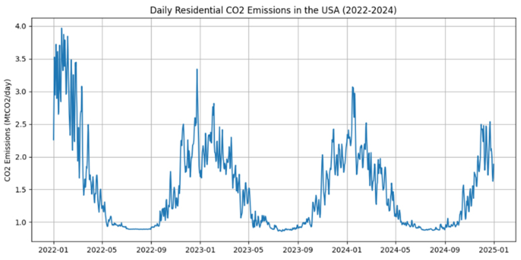
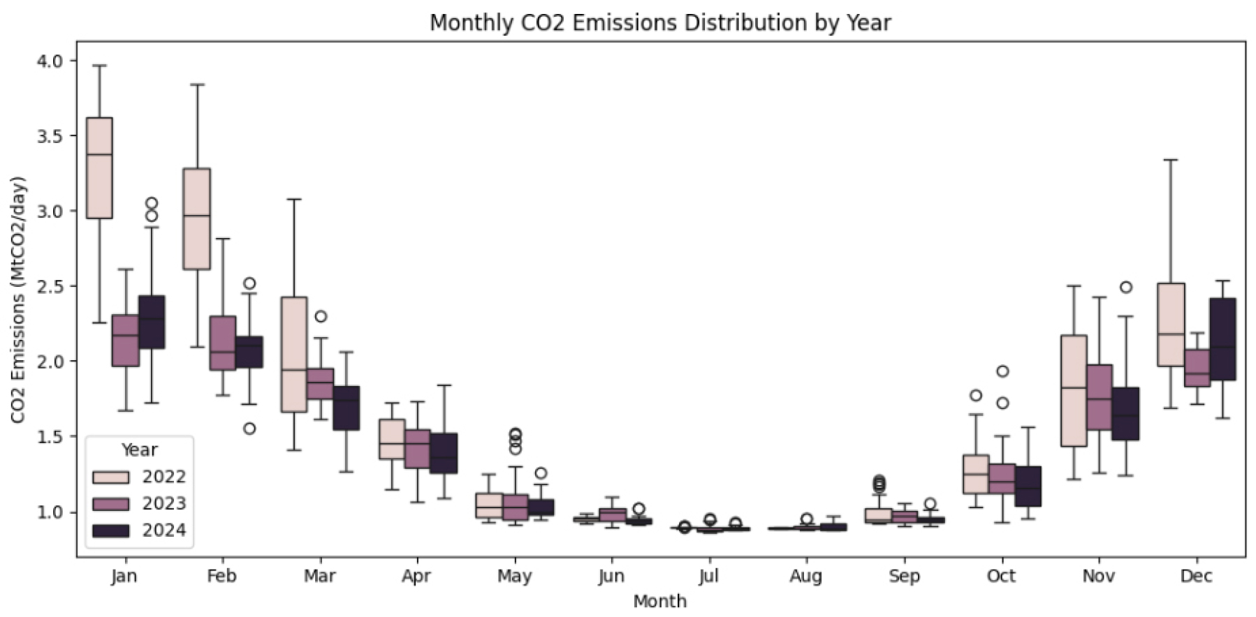
Figure 2 presents a box plot analysis of monthly CO2 emissions from the U.S. residential sector between 2022 and 2024, revealing pronounced seasonal variability. Elevated emission levels (median range: 2.0–3.0 MtCO2/day) are observed during colder months (January–March, November–December), attributable to heightened heating demands. Conversely, emissions decline significantly (below 1.5 MtCO2/day) from April to September, coinciding with reduced energy consumption. A marginal reduction in emissions during 2024 suggests potential improvements in energy efficiency, while sporadic outliers may reflect anomalous weather events. These findings underscore the dominant influence of seasonal climatic conditions on residential energy use, with deviations likely linked to transient meteorological extremes.
Data Preprocessing
Data Cleaning:
The dataset required no imputation for missing data, as it was complete with no missing values.
Lag Feature Creation:
A key preprocessing enhancement was the creation of a lag feature (lag_1), which incorporates the previous day’s CO2 emissions as a predictor variable. For a time series of CO2 emissions {y1,y2,...,yT}, the lag-1 feature at time t is mathematically defined as:
The resulting input–output structure conforms to the supervised learning paradigm, where the input vector Xt at time t includes xlag_1,t and the corresponding target value is yt. This temporal feature provides the models with historical context, allowing them to identify sequential patterns and correlations between consecutive days’ emissions.
Time-Based Data Splitting:
In time-series modeling, maintaining the chronological integrity of observations is essential to avoid forward-looking bias. Therefore, rather than employing random sampling, a time-based holdout validation approach was implemented. The data were partitioned into a training set and a testing set based on calendar date.
•The training set consisted of the first 730 daily observations, representing the period from January 1, 2022, to December 31, 2023.
•The testing set comprised the remaining 365 observations, spanning January 1, 2024, to December 30, 2024.
This partitioning ensures that the test data encompass all seasonal cycles, thereby enhancing the generalizability and temporal robustness of the forecasting models. The formal representation of the partition is given by:
where Xi represents the input features on day i , yi denotes the corresponding CO2 emission, and T = 1095 is the total number of samples.
Machine learning models
1. Decision Tree:
A DT is a well-established and efficient methodology for classification and regression tasks, extensively applied across numerous scientific domains, including the construction industry. The method functions by traversing instances through a hierarchical tree structure, initiating at the root and concluding at a leaf node, which determines the instance’s final classification or predicted value. At each node, a decision is made based on a specific attribute, with the information gain calculated using entropy, a measure of uncertainty for a discrete random variable, where C represents the set of target classes. For a dataset D, the entropy is defined as equation (4).
• is the proportion of samples in class
• is the total number of classes.
When an attribute Ai with v values partitions D into ν subsets {D1, D2, …, Dν}, the expected entropy is computed as equation 5 and the information gain is derived as equation 6.
• is the number of observations in subset
• is the total number of observations in the original dataset.
In this study, the DT model was implemented using the “DecisionTreeRegressor” class from the scikit-learn library. Key hyperparameters, such as maximum depth and minimum samples per split, were optimized through grid search applied exclusively on the training data to preserve temporal ordering and avoid data leakage.
2. Random Forest:
Extending the DT framework, RF employs an ensemble of independent, de-correlated decision trees, where each tree produces a prediction for an instance, and the final output is determined via majority voting for classification or averaging for regression [17]. To ensure tree independence, each tree is constructed using a distinct bootstrap sample, and at each node, a random subset of m variables is selected from the total input variables to identify the optimal split. Node impurity is evaluated using metrics such as the misclassification rate, Gini index, and cross-entropy (equations 7–9), where k(m) denotes the majority class in node m, Pmk represents the proportion of class k observations in node m, and yi is the class of observation i; notably, the Gini index, which quantifies the probability of misclassification if an instance were labeled randomly according to the node’s label distribution, and cross-entropy are more sensitive to variations in node probabilities than the misclassification rate.
The Random Forest model was developed using the “RandomForestRegressor” class from scikit-learn. Hyperparameter tuning—such as the number of estimators, maximum tree depth, and minimum leaf size—was conducted using grid search on the training set only, in order to maintain the integrity of the time-series structure and ensure generalizability.
3. Ridge Regression:
Ridge Regression is a linear regression technique that addresses multicollinearity (high correlation among independent variables) and overfitting by introducing a regularization term to the loss function. This regularization term penalizes large coefficients, thereby shrinking them towards zero. Ridge Regression is particularly useful when dealing with datasets where the number of predictors is large relative to the number of observations, or when predictors are highly correlated.
The Ridge Regression model modifies the ordinary least squares (OLS) objective function by adding a penalty proportional to the sum of the squared coefficients. The Ridge Regression loss function is given by:
Where:
•yi is the actual value of the dependent variable for the ith observation.
•ŷi is the predicted value of the dependent variable for the ith observation, calculated as ŷi=β0+β1xi1+β2xi2+⋯+βpxip.
•β0, β1, …, βp are the regression coefficients.
•λ is the regularization parameter, which controls the strength of the penalty.
•n is the number of observations.
•p is the number of predictors.
In this study, Ridge Regression was implemented using scikit-learn’s “Ridge” class, with hyperparameters optimized through cross-validation applied only to the training set, thereby preserving temporal sequence and preventing data leakage.
4. Gradient Boosting:
GB operates by sequentially constructing regression trees, where each new tree is designed to correct the residual errors of the preceding ones. The process starts with an initial regression tree, followed by iterative tree-building steps that progressively partition the data into smaller subsets, with each subsequent tree trained to minimize the errors identified in the previous iteration. This iterative process persists until a predefined number of trees is reached or further improvements in model fit cease, while a learning rate is applied to regulate the contribution of each tree, mitigating overfitting by enhancing generalization, as a smaller learning rate reduces the impact of individual trees on the final model. Key parameters optimized to enhance the performance of the GB model include the maximum depth of the trees, the number of estimators, and the learning rate, ensuring a balance between accuracy and robustness.
In this study, the GB model was implemented using the “GradientBoostingRegressor” class from the scikit- learn library. Hyperparameter tuning was performed via grid search on the training dataset, with cross-validation applied in a time-aware manner to ensure the temporal integrity of the data was preserved.
5. Support Vector Regression:
SVR, rooted in statistical learning theory, transforms input data into a higher-dimensional space using kernel functions to identify an optimal hyperplane that maximizes the margin of tolerance, balancing complexity and accuracy. The model, expressed via Lagrange multipliers (α_i), kernel function K(x_i, x), and bias term b (equation 10), uses linear and RBF kernels to capture linear and nonlinear patterns in daily CO2 emissions, selected for their simplicity and effectiveness. Performance is optimized by tuning the kernel, epsilon (ε) for tolerance, and regularization parameter C, which balances training error and model simplicity to prevent overfitting.
Where:
• is the predicted output,
• represents the support vectors,
• are the Lagrange multipliers estimated during training,
• is the kernel function, which maps the data to a higher-dimensional space,
• is the bias term.
In this study, the “Radial Basis Function” kernel was selected due to its capability to model complex, nonlinear emission patterns while remaining computationally efficient. Model performance was tuned by optimizing three key hyperparameters:
•The regularization parameter C, which controls the trade-off between training error and model complexity.
•The kernel coefficient γ, which defines the influence of individual training examples in the RBF kernel.
•The epsilon ε, which specifies the allowable deviation from the true value within which predictions incur no penalty.
6. XGBoost:
Extreme Gradient Boosting (XGBoost) is a fast, scalable implementation of gradient boosting that constructs an ensemble of regression trees sequentially, each correcting the residuals of the previous ones. It incorporates a second-order Taylor approximation of the loss function for more precise optimization and integrates regularization to control model complexity and reduce overfitting. Designed for efficiency, XGBoost supports parallel computation, column subsampling, and optimized tree pruning, making it particularly effective for time-series forecasting tasks such as CO2 emissions prediction.
The performance of the model is governed by several hyperparameters, including:
•Learning rate (𝜂)— scales the contribution of each tree to the final prediction,
•Maximum tree depth — determines the complexity of each tree, and
•Number of estimators — defines the total number of trees in the ensemble.
In this study, the XGBoost model was implemented using the “XGBRegressor’ class from the XGBoost Python library. The model’s hyperparameters were tuned via grid search exclusively on the training data, preserving the temporal structure of the time-series and ensuring the robustness and generalizability of the results.
Deep Learning model
Long Short-Term Memory:
LSTM is a Recurrent Neural Network (RNN) architecture well-suited for modeling time-series data due to its ability to capture long-range temporal dependencies. Its inclusion in this study is motivated by its proven effectiveness in learning from sequential patterns, which are inherent in daily CO2 emission data. The LSTM model in this work was designed with a combination of recurrent and dense layers, with dropout applied to enhance generalization. The model was trained using the Adam optimizer and the Mean Squared Error (MSE) loss function. Early stopping was implemented to prevent overfitting by halting training once the validation performance ceased to improve.
Input sequences were structured using a 7-day look- back window, enabling the model to learn from short- term historical emissions. Prior to training, all features were scaled to a [0, 1] range using MinMaxScaler to support numerical stability and faster convergence. The entire model pipeline was implemented using the TensorFlow/Keras deep learning framework.
SHAP Analysis
To enhance the interpretability of the machine learning models and validate feature contributions, SHAP (SHapley Additive exPlanations) analysis was employed. SHAP provides a unified framework for quantifying the impact of each input variable on the model’s predictions by computing Shapley values derived from cooperative game theory. For tree-based models (e.g., DT, Random Forest, Gradient Boosting, XGBoost), SHAP’s TreeExplainer was used, while KernelExplainer was applied for linear and support vector models. Each model’s SHAP values were computed using a representative subset of test samples, enabling both summary plots and feature importance rankings. For the LSTM model, GradientExplainer was utilized with background and test samples constructed from the temporally ordered sequences. SHAP values were aggregated across time steps to evaluate temporal feature importance and to visually capture how recent emission values influenced predictions.
Model Evaluation Metrics
To assess the predictive performance of the models, four widely used regression evaluation metrics were employed: Mean Squared Error (MSE), Root Mean Squared Error (RMSE), Mean Absolute Error (MAE), and the Coefficient of Determination (R²). These metrics are briefly described in Table 1.
Table 1.
Description of Model Evaluation Metrics
Result and Discussions
Six traditional machine learning models— DT, RF, Ridge Regression, Gradient Boosting, SVR and XG Boost —alongside a LSTM deep learning model, were developed and evaluated to forecast residential CO2 emissions. The predictive performance of each model was assessed using widely accepted evaluation metrics, including MSE, RMSE, MAE, and R², computed on the testing dataset.
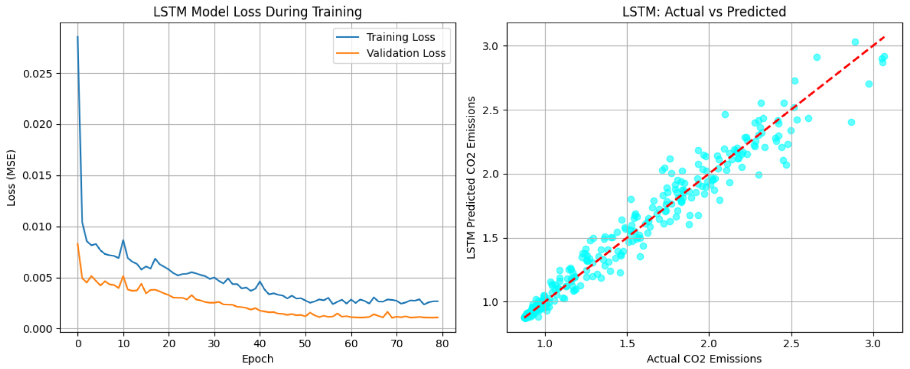
Figure 3 provides diagnostic insights into the training and predictive performance of the LSTM model. The left panel shows training and validation loss curves over 80 epochs, both steadily decreasing and stabilizing without signs of overfitting. This indicates effective model convergence and generalization. The right panel displays actual versus predicted CO2 emissions, with data points closely aligned along the 45-degree reference line, confirming the model’s high accuracy on unseen data. These diagnostics visually support the LSTM’s quantitative superiority among all models evaluated.
A comparative analysis of the models based on model evaluation metrics revealed the following (Figure 4 and Table 2):
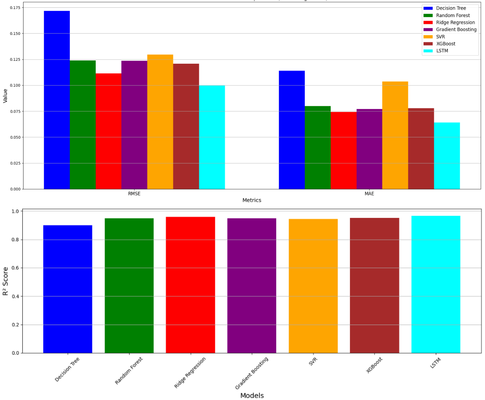
Table 2.
Model Comparison based on Metrics
•LSTM demonstrated the highest predictive accuracy among all models, achieving the lowest MSE (0.0100), RMSE (0.1000), and MAE (0.0641), along with the highest R² value of 0.9662. These results indicate that LSTM effectively captured complex temporal patterns, yielding the most reliable predictions with minimal error.
•Ridge Regression ranked second, with strong performance across all metrics—MSE of 0.0124, RMSE of 0.1115, MAE of 0.0743, and an R² of 0.9579—demonstrating robust generalization and high explanatory power.
•XGBoost followed closely, showing competitive results with an MSE of 0.0146, RMSE of 0.1208, MAE of 0.0778, and an R² of 0.9505, indicating consistent performance in capturing nonlinear relationships.
•Gradient Boosting exhibited similar accuracy, with an MSE of 0.0153, RMSE of 0.1235, MAE of 0.0771, and R² of 0.9483. Its predictive error remained low, although slightly higher than XGBoost.
•RF also delivered reliable results (MSE: 0.0154, RMSE: 0.1240, MAE: 0.0801, R²: 0.9479), performing comparably to other ensemble methods but with marginally higher error.
•SVR showed moderate performance, yielding a Root Mean Squared Error of 0.1296 and an R² of 0.9430. However, its higher Mean Squared Error of 0.0168 and Mean Absolute Error of 0.1037 indicated limited precision in individual forecasts.
•The DT model underperformed relative to the others, yielding the highest error values (MSE: 0.0294, RMSE: 0.1716, MAE: 0.1141) and the lowest R² (0.9002), reflecting limited generalization capacity and increased sensitivity to data fluctuations.
Visualizations of the predicted CO2 emissions versus actual values, along with residual plots for each model, were generated to further assess model fit (Figure 5 and 6). Figure 5 illustrates the alignment between actual daily CO2 emissions and predicted values produced by various machine learning models. Among the compared methods, the LSTM model demonstrated the most consistent and accurate tracking of emission patterns throughout the year, particularly during periods of rapid fluctuation and seasonal peaks. Its ability to incorporate temporal dependencies enabled it to capture both long-term trends and short-term anomalies with notable precision. Ensemble models such as XGBoost, Gradient Boosting, and Random Forest also closely followed the overall emission trajectory. Their performance reflects the models’ strength in capturing non-linear relationships and seasonal cycles, although their predictions exhibited slightly greater variability compared to LSTM. Ridge Regression showed strong agreement with the actual data, reinforcing the presence of a substantial linear component in the emissions pattern. In contrast, SVR tended to underestimate peak emissions, particularly during high-demand winter months, indicating limitations in its ability to model extreme values. The Decision Tree model showed less stability, with more erratic predictions and reduced ability to generalize across varying temporal patterns. The results underscore the effectiveness of deep learning approaches for time-series prediction in environmental data contexts, while also highlighting the continued relevance of well-tuned ensemble and linear models in capturing key structural patterns in CO2 emissions.
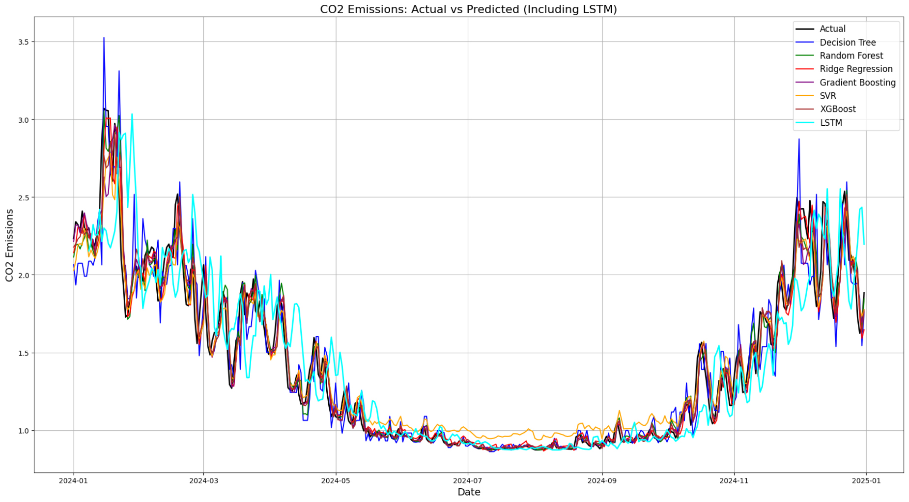
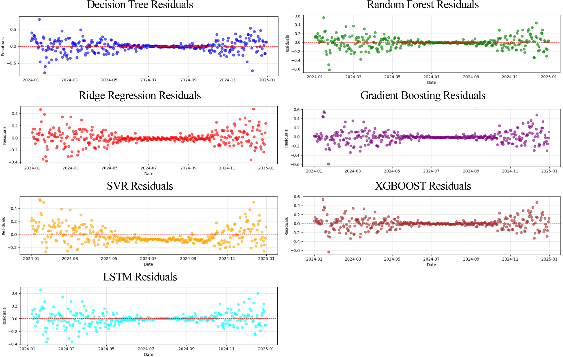
Figure 6 presents residual plots for all models, offering insights into the distribution and patterns of prediction errors across the 2024 test period. Ideally, residuals should be randomly scattered around zero, indicating unbiased predictions with consistent variance. The LSTM model shows tight residuals mostly clustered around zero, particularly from late spring through early fall. While there is slight widening during high- emission periods (e.g., winter), the distribution remains symmetric with no systematic bias, indicating strong temporal learning and robustness throughout the year. XGBoost also demonstrates relatively consistent and narrow residuals, with most points centered close to the zero line. Some minor fluctuations appear in late months, but the errors remain balanced, suggesting effective generalization even during emission spikes. SVR, on the other hand, shows a clear asymmetric bias. Residuals tend to be negative in mid-year and shift to positive toward the end of the year, reflecting systematic underestimation during summer and overestimation in winter. This indicates that SVR fails to fully capture seasonal shifts. Gradient Boosting and Random Forest both show well-centered residuals with slightly more dispersion than LSTM or XGBoost. These models handle the majority of the test period well, but show increased variability during the cold months, likely due to more volatile emission levels. The Ridge Regression model exhibits a dense central residual band with some spread during winter. The pattern is still symmetric and lacks major outliers, suggesting good linear fit with mild seasonal sensitivity. In contrast, the DT model shows the most erratic residual pattern, especially early in the year and again in the final quarter. Residuals fluctuate sharply with no clear structure, pointing to instability and reduced generalization under dynamic conditions. Taken together, these residual plots confirm the superior performance of the LSTM model, which shows the most compact, unbiased error distribution. Among traditional models, XGBoost exhibits the cleanest residual behavior, followed closely by Gradient Boosting and Ridge Regression. In contrast, DT residuals are highly scattered, and SVR demonstrates systematic seasonal bias, reflecting their limitations in modeling time- dependent and non-linear emission patterns.
The SHAP analysis provided crucial insights into the interpretability of the machine learning models for daily residential CO2 emissions prediction. Across all traditional machine learning models, the analysis revealed a pronounced dominance of the lag_1 feature (previous day’s emissions), which exhibited an average SHAP importance value of 0.6447. This finding strongly suggests that residential CO2 emissions demonstrate significant day-to-day autocorrelation, where the most recent historical observation serves as the primary predictor for future values. The temporal features showed varying degrees of importance, with the year feature (average importance: 0.0255) and month feature (average importance: 0.0226) contributing moderately to model predictions, while day and dayofweek features exhibited minimal influence on the prediction outcomes (Figure 7).
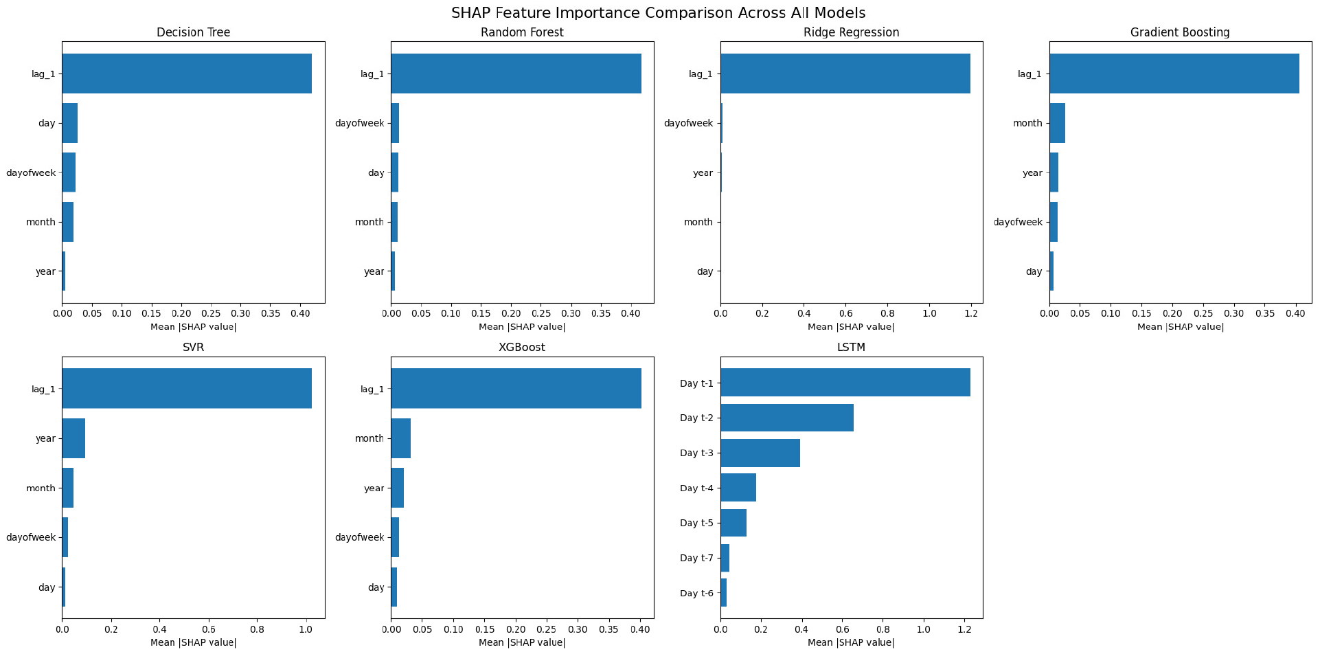
The LSTM model’s SHAP analysis revealed distinctive temporal importance patterns that differentiate it from traditional machine learning approaches. Using gradient-based importance analysis, a clear temporal decay pattern was observed where the most recent time step (t-1) demonstrated the highest importance value of 1.2282, with importance decreasing progressively for earlier time steps. This pattern indicates that the LSTM model successfully captures the strong short- term dependencies inherent in residential CO2 emissions data. The model’s ability to assign differential weights to historical observations based on their temporal proximity represents a significant advantage over traditional models that rely solely on fixed-lag features.
The SHAP analysis uncovered consistent patterns across different model categories. Tree-based models (DT, RF, Gradient Boosting, and XGBoost) demonstrated remarkably uniform feature importance distributions, with all models heavily relying on the lag_1 feature for predictions. This consistency suggests that ensemble methods, despite their complexity, converge on similar feature utilization patterns when predicting CO2 emissions. Linear models (Ridge Regression) and SVR showed slight variations in feature weighting but maintained the same hierarchical importance structure. The uniformity of feature importance across diverse algorithms reinforces the robustness of the findings regarding the autoregressive nature of residential CO2 emissions.
The dominance of autoregressive features in this analysis has important implications for CO2 emissions forecasting strategies. The strong predictive power of the previous day’s emissions (lag_1) across all traditional models indicates that residential CO2 emissions follow highly predictable short-term patterns. This predictability likely stems from consistent human behavior patterns, regular household activities, and the thermal inertia of residential buildings. The moderate importance of seasonal features (year and month) suggests that while long-term trends and seasonal variations exist, they play a secondary role compared to immediate historical values in daily prediction tasks.
The superior performance of the LSTM model (RMSE: 0.1000) compared to traditional machine learning approaches (RMSE range: 0.1115-0.1716) can be directly attributed to its ability to process sequential information without explicit feature engineering. While traditional models are constrained by predetermined lag features, the LSTM dynamically learns temporal dependencies across multiple time steps. The SHAP analysis confirmed that the LSTM effectively utilizes a seven-day historical window, with each day contributing differentially to the final prediction. This architectural advantage allows the LSTM to capture complex non-linear temporal patterns that may be missed by models relying on single-lag features.
Conclusions
Accurate prediction of daily residential CO2 emissions is essential for governmental initiatives aimed at mitigating global warming, particularly in the United States, where the residential sector significantly contributes to national emissions. Among the models tested, the Long Short-Term Memory neural network demonstrated the highest forecasting accuracy, achieving the lowest Root Mean Squared Error (0.1000) and the highest coefficient of determination (R² = 0.9662). This result underscores the LSTM’s capacity to capture short-term temporal dependencies in emissions data, particularly during periods of high variability.
In contrast, while Ridge Regression and XGBoost demonstrated competitive performance with relatively low error rates and strong generalization, they were constrained by their reliance on engineered lag features and could not fully exploit the temporal structure of the data. SHAP analysis reinforced these findings, revealing that all traditional models heavily depended on the previous day’s emissions as the dominant predictor, whereas the LSTM model dynamically assigned importance across a 7-day sequence, offering a more nuanced understanding of emission dynamics. Furthermore, the SHAP analysis enhances the interpretability of black-box models, providing valuable insights for practical applications. The clear dominance of recent historical data in predictions suggests that real-time monitoring systems with even short historical windows can achieve high prediction accuracy. The minimal importance of day-of-week features indicates that residential CO2 emissions may not follow strong weekly patterns, possibly due to the averaging effects across diverse household types or the increasing prevalence of flexible work arrangements. For stakeholders implementing CO2 monitoring systems, these findings suggest that investing in high-frequency, recent data collection may yield better returns than extensive historical databases.
These findings are consistent with prior research in environmental forecasting, which highlights the strong performance of deep learning models—particularly LSTM—for sequential prediction tasks. Kumari and Singh (2022) found LSTM to be the most accurate among six models for forecasting national CO2 emissions in India. Similarly, Ajala et al. (2024) showed that LSTM and its variants performed among the top models for CO2 emissions across major regions. However, their study also emphasized that ensemble-based machine learning models offered a practical trade-off between accuracy and computational efficiency, making them preferable for operational use.
While this study provides valuable insights, several limitations should be acknowledged. The gradient-based approach used for LSTM interpretation may not capture all complex interactions within the recurrent architecture. Additionally, the analysis focuses on individual feature importance without fully exploring feature interactions, which may play crucial roles in prediction accuracy. Future research could employ more sophisticated interpretability methods, such as attention mechanisms in transformer architectures, to provide deeper insights into temporal pattern recognition. Furthermore, investigating the stability of these feature importance patterns across different geographical regions, building types, and seasonal conditions would enhance the generalizability of these findings.
