Soil structure interaction using Lyzmer type viscous dampers and domain reduction method with flexibility-based model for an existing structure and comparison between 3D and 2D model without Soil modelization

Sabah Moussaoui; Mourad Belgasmia

doi:10.22712/susb.20210002

Preview

General Article

International Journal of Sustainable Building Technology and Urban Development. 31 March 2021. 2-13
https://doi.org/10.22712/susb.20210002

Soil structure interaction using Lyzmer type viscous dampers and domain reduction method with flexibility-based model for an existing structure and comparison between 3D and 2D model without Soil modelization

Sabah Moussaoui¹

Mourad Belgasmia²^*

¹Assistant, Department of Civil Engineering, Setif 1 University Algeria, Setif

²Dr, Department of Civil Engineering, Setif 1 University Algeria, Setif

^{*Corresponding Author}

ABSTRACT

The main goal of this article is to analyze computational model that concerns the structure and only a small adjacent part of subsoil using Domain Reduction Method (DRM) and taking into account the absorbing boundaries Lyzmer type viscous dampers with flexibility-based model, by the use of force-based element, and single element for 3D and 2D model. Through this method, the size of the problem to be solved is substantially reduced. Another goal of this article is a comparison between pushover curve of 3D and 2D model under an imposed displacement at the top of the structure using flexibility based model.

Keywords

lyzmer viscous dampers

soil structure interaction

seismic load

single media

domain reduction method

flexibility based model

MAIN

Introduction
Equations of motion for single-phase media
Absorbing boundaries (single-phase)
Viscos force vector
Requirements for time and space discretization
Domain reduction method and flexibility based model
Seismic input
Static nonlinear study of an existing building using flexibility based model
Ultimate load analysis under imposed displacement 2D equivalent and 3D comparison
Soil Structure 2D and 3D model using Lyzmer type viscous damper
Results and discussion
Conclusion

Introduction

In order to verify the existing earthquake structures; an alternative nonlinear method to solve the dynamic equation in time emerged in the late 1990s, which is now documented in the various standards in force. The “pushover” method, based on deformations [1], allows to define a target displacement by comparing a demand spectrum (provided by the standards) and a capacity spectrum (obtained by expressing the displacement of the structure according to the monotonous increase of a horizontal force).

This method, now applied to structures only, is extended here to the surrounding soil-structure system. In the early 2000s, it still seems unlikely to be able to solve a seismic verification problem in the near future by means of a real time resolution on a PC. In the ten years later, the resolution of the equation of dynamics on a nonlinear involving soil-structure interaction is nevertheless possible [2]. Thanks among other things to Domain Reduction Method (DRM), proposed by [3], which allow dividing the problem into two models: linear, often essentially one-dimensional, providing seismic input (free-field motion). Other nonlinear, and limited to the proximity of the analyzed structure (about 50’000 degrees of freedom).

It is now imperative to optimize our the way of thinking whether in the design or in a numerical model of the structure in order to get as close as possible to the real behavior of the structure [4].

Equations of motion for single-phase media

In time history analysis, with a given solution for accelerations, velocities and displacements at time $t_{n}$ , we seek for the solution at time $t_{n + 1}$ by solving the following discretized (in time and space) equations of motion.

(1)

M a + C v + N (d) = F_{e x t}

Where nodal accelerations, velocities and displacements are denoted by $a, v$ and $d$ , respectively. The $N (d)$ is a nonlinear vector of internal forces, the $F_{ext}$ is the external force vector, $M$ is the mass matrix (lumped or consistent) and $C$ is the damping matrix.

(2)

C = α_{0} [M] + β_{0} [K]

(3)

\{\begin{matrix} ξ_{1} \\ ξ_{2} \end{matrix}\} = 0.5 [\begin{matrix} \frac{1}{ω_{i}} & ω_{j} \\ \frac{1}{ω_{j}} & ω_{j} \end{matrix}] \{\begin{matrix} α_{0} \\ β_{0} \end{matrix}\}

Absorbing boundaries (single-phase)

Viscos force vector

The resulting damping force vector that is added to the right hand side is defined as follows:

(4)

F^{v} = - \int_{Γ}^{} N^{t} σ^{s} d Γ

In the above equation, N is a matrix of standard shape functions and $σ^{s}$ is a viscous stress defined as:

(5)

σ = - \{\frac{1}{c_{p}} (λ_{s} + 2 μ_{s}) n n^{t} + \frac{μ_{s}}{c_{s}} (t_{1} t_{1}^{t} + t_{2} t_{2}^{t})\} V^{s}

The corresponding shear and dilatational wave velocities are denoted respectively by :

(6)

C_{s} = \sqrt{\frac{G}{ρ}} C_{p} = \sqrt{\frac{λ + 2 G}{ρ}}

While solid velocity vector at a given point by $v^{s}$ , the normalized normal and tangential vectors are denoted by $n$ and $t_{1}, t_{2}$ respectively. Note that Lysmer type viscous dampers are the simplest elements that help to cancel wave reactions from domain boundaries. However, only in some certain situations, the elements give results with high accuracy or even exact. This strongly depends on the angle of wave incidence. Viscous dampers can be generated at the macro modeling (which is meaningful for deformation or deformation and Flow transient dynamics analyses) or finite element level, it will be created on edges of the mesh of continuum elements once the virtual and then the real mesh in the continuum subdomain is created.

Requirements for time and space discretization

In order to trace wave propagation in the medium we need approximately 10 nodes per wavelength. The mesh size depends on the maximum frequency $f_{\max}$ which will be represented. For typical seismic application $f_{\max}$ is limited up to 10 Hz. Hence, the maximum mesh size should be smaller than.

(7)

h^{e} \leq \frac{λ}{10} = \frac{v}{10 f_{m a x}}

In the most cases υ is taken as shear wave velocity.

Size of the applied time step, even for implicit integration schemes, is limited to a certain value too. This is so due to the fact that the smallest fundamental period of vibration needs to be represented by at least 10 points (same amount as for the spatial discretization). Hence, the time step limitation can be formulated as follows :

(8)

Δ t \leq \frac{h^{e}}{v}

Domain reduction method and flexibility based model

As long as the modeling of the soil with the structure generates a finite element model whose mesh is very important, therefore the size of the matrix is so. It is imperative to use methods, which are effective in terms of computation and meshing either for structure or for soil bearing this later.

The force-based method formulation is based on force interpolation that satisfies the balance of the element thing that ranks it to flexibility-based elements category; offering thus undeniable advantages over the existing displacement-based approach. One of the first advantages is that there are no discretization error, and all the equations are perfectly satisfied. Add to that the drastic reduction in number of elements structure for discretization [5], [6].

In terms of the infra-structure part (soil), another elegant method so-called, Domain Reduction Method has seen the day with [3]. This method reduce the size of the problem to be solved , this a part of the subsoil surrounding the super structure is taken into consideration, displacements, velocities, accelerations are stored at nodes that belong to the boundary layer of elements.

These quantities are used to compute effective forces that are applied through the boundary between exterior and interior domain. The detailed derivation of the approach can be found in [2], [7].

Seismic input

Seismic input is given as imposed displacements or accelerations of the ground. Independently of the input format, the solving algorithms can find the solution in terms of accelerations, displacements, or velocities.

As the problem to be solved is nonlinear, an iterative procedure is needed; Newton-Raphson Nonlinear implicit Newmark algorithm is one of the most common in transient dynamics. The following implementation scheme is given by [8], used here to linearize the problem. Considering the static procedure first. If superscript i+1 indicates iterations, in the vicinity of the displacement $d_{n + 1}^{i + 1}$ .

(9)

N (d_{n + 1}^{i + 1}) ≅ N (d_{n + 1}^{i}) + \frac{dN}{dd} Δd = N (d_{n + 1}^{i}) + K_{T} Δd

Hence:

(10)

\{\begin{cases} K_{T} Δd = F_{n + 1} - N (d_{n + 1}^{i}) \\ d_{n + 1}^{i + 1} = d_{n + 1}^{i} + Δd \end{cases} (with d_{n + 1}^{0} = d_{n})

Convergence is reached when:

(11)

∥ F_{n + 1} - N (d_{n + 1}^{i + 1}) < t o l e r a n c e ∥

Remarks:

The following algorithmic alternative are possible

- Update K at each step and iteration: full Newton-Raphson

- Opportunistic update: modified Newton-Raphson

- $K_{T} = K_{0}$ : constant stiffness algorithm

Considering the dynamics procedure in terms of incremental displacements $Δd$ let’s define:

(12)

N^{*} (d) = Ma + Cv + N (d) K^{*} = (\frac{{dN}^{*}}{dd}) = \frac{M}{{Δt}^{2} β} + \frac{γ}{Δtβ} C + K

Initialization

(13)

d_{0} = d (0) v_{0} = v (0)

For every Δt

Compute predictors

(14)

{\tilde{d}}_{n + 1} = d_{n} + Δ t v_{n} + (1 - 2 β) \frac{Δ t^{2}}{2} a_{n} {\tilde{v}}_{n + 1} = v_{n} + (1 - 2 γ) a_{n} d_{n + 1}^{i = 0} = {\tilde{d}}_{n + 1} v_{n + 1}^{i = 0} = {\tilde{v}}_{n + 1} a_{n + 1}^{i = 0} = 0

For every Δd

Solve

(15)

Δ F_{n + 1}^{i} = F_{n + 1} - N^{*} (d_{n + 1}^{i}) K_{n + 1}^{i} = F_{n + 1} - N^{*} (d_{n + 1}^{i}) {ΔF}_{n + 1}^{i} = F_{n + 1} - N^{*} (d_{n + 1}^{i}) K_{T}^{* i} Δd = {ΔF}_{n + 1}^{i} d_{n + 1}^{i + 1} = d_{n + 1}^{i} + Δd

Compute correctors

(16)

a_{n + 1}^{i + 1} = \frac{a_{n + 1}^{i + 1} - {\tilde{d}}_{n + 1}}{∆ t^{2} β} v_{n + 1}^{i + 1} = {\tilde{v}}_{n + 1} + ∆ t γ a_{n + 1}^{i + 1}

Next iteration

if $∆ F_{n + 1}^{i} > T O L E R A N C E \Rightarrow i = i + 1$

Next time step

if $t < T_{m a x} \Rightarrow n = n + 1 \sum_{}^{}$

Remarks:

The following algorithmic alternative are possible

1 Update K at each step and iteration: full Newton-Raphson

2 Opportunistic update: modified Newton-Raphson

3 $K_{T}$ = $K_{0}$ : constant stiffness algorithm

Static nonlinear study of an existing building using flexibility based model

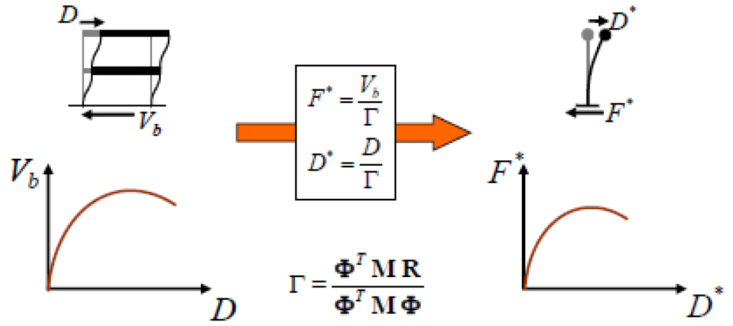
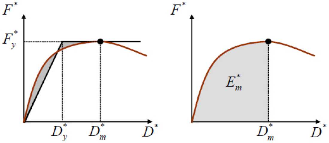
In this section a graphic summary of static nonlinear method is given first (see Figures 1 & 2) and then the algorithm that goes with it.

https://cdn.apub.kr/journalsite/sites/durabi/2021-012-01/N0300120101/images/Figure_susb_12_01_01_F1.jpg

Figure 1.

Capacity curve: transformation from response of MDOF to equivalent SDOF.

https://cdn.apub.kr/journalsite/sites/durabi/2021-012-01/N0300120101/images/Figure_susb_12_01_01_F2.jpg

Figure 2.

Bilinearization of the SDOF capacity curve.

Seismic demand assesment algorithm :

A. Given $D_{m}^{*} F_{y}^{*}$ from the bilinearized capacity spectrum :

B. set : $D_{y}^{*} = 2 (D_{m}^{*} - \frac{E_{m}^{*}}{F_{y}^{*}}); T^{*} = 2 π \sqrt{\frac{m * D_{y}^{*}}{F_{y}^{*}}}; q_{u} = \frac{S_{A e} (T^{*})}{F_{y}^{*} / m^{*}}$

C. Reduce spectrum

If ( $T^{` *} < T_{C} \sum_{}^{}$ )

$q_{μ} \leq 1 \Rightarrow D_{t}^{*} = S_{D e} (T^{*})$ Response remain elastic

$q_{μ} > 1 \Rightarrow D_{t}^{*} = \frac{S_{D e} (T^{*})}{q_{μ}} μ$ ; with $μ = 1 + (q_{μ} - 1) \frac{T_{C}}{T^{` *}}$

else ( $T^{` *} \geq T_{C}$ )

$q_{μ} \leq 1 \Rightarrow D_{t}^{*} = S_{D e} (T^{*})$ Response remain elastic

$q_{μ} > 1 \Rightarrow D_{t}^{*} = \frac{S_{D e} (T^{*})}{q_{μ}} μ$ ; with $μ = q$

D. Check

If $|D_{m}^{*} - D_{t}^{*}| < t o l$ stop

Else

Set : $D_{m}^{*} = D_{t}^{*}$

Go to A.

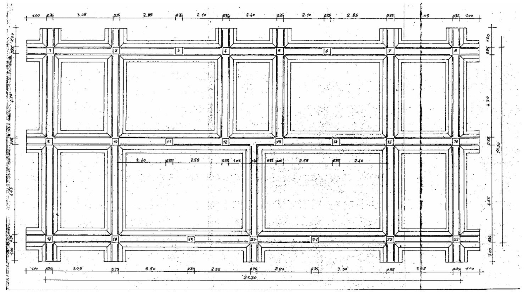
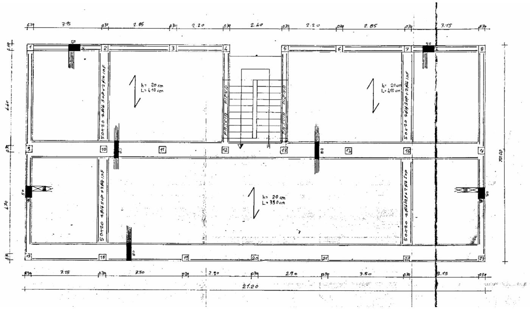
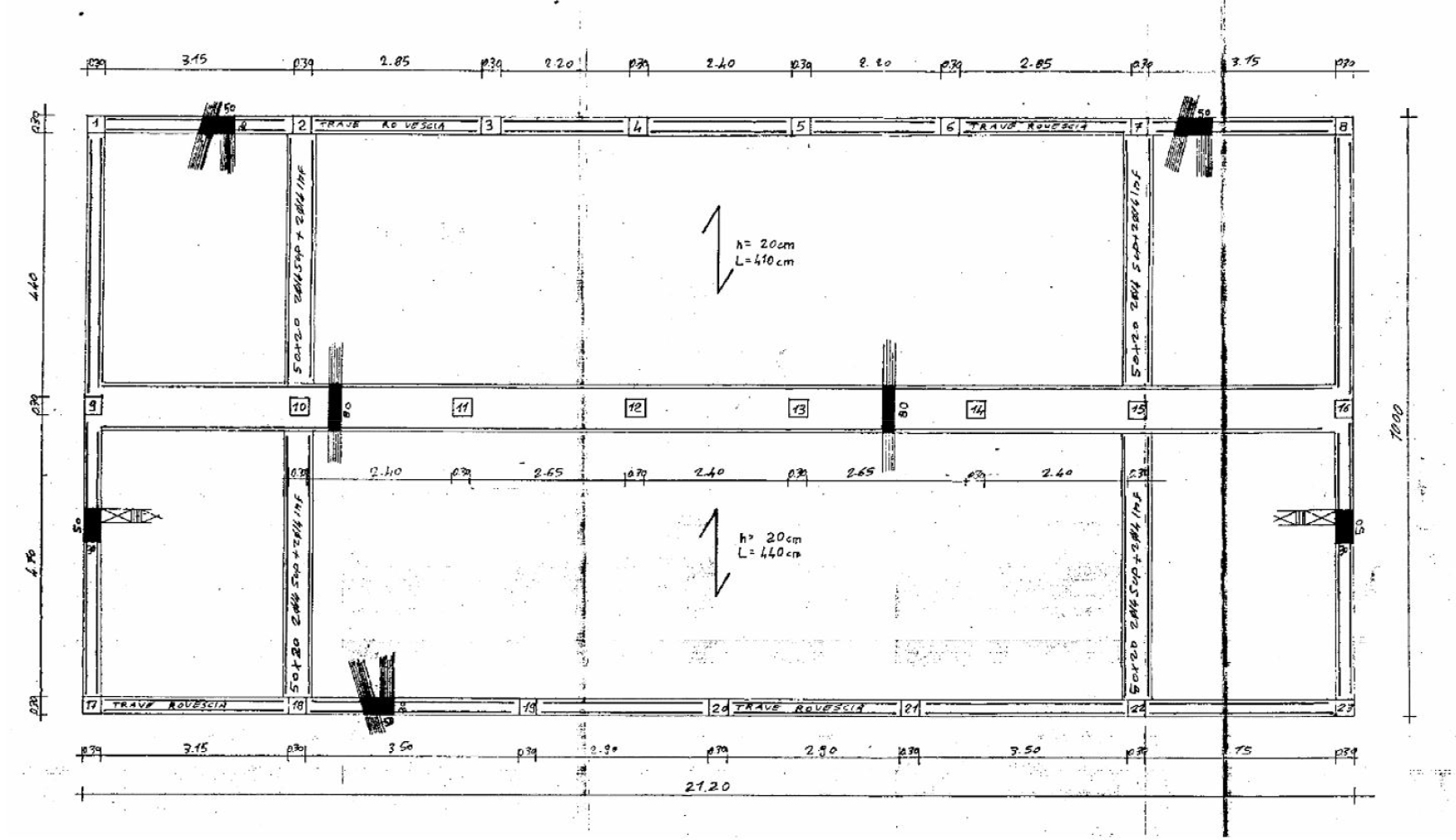
An existing three-storey is a residential two-storey building with reinforced concrete building is studied using the nonlinear frame analysis capabilities of Z_Soil. It is a good example of residential buildings of the 70’s and 80’s in Italy [9] using [10]. Foundation, floor and roof plans are shown in Figure 3, 4, 5.

https://cdn.apub.kr/journalsite/sites/durabi/2021-012-01/N0300120101/images/Figure_susb_12_01_01_F3.jpg

Figure 3.

Foundation building plan.

https://cdn.apub.kr/journalsite/sites/durabi/2021-012-01/N0300120101/images/Figure_susb_12_01_01_F4.jpg

Figure 4.

First and second floor building plan.

https://cdn.apub.kr/journalsite/sites/durabi/2021-012-01/N0300120101/images/Figure_susb_12_01_01_F5.jpg

Figure 5

Third level and roof building plan.

Ultimate load analysis under imposed displacement 2D equivalent and 3D comparison

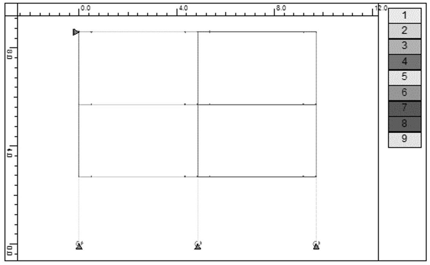
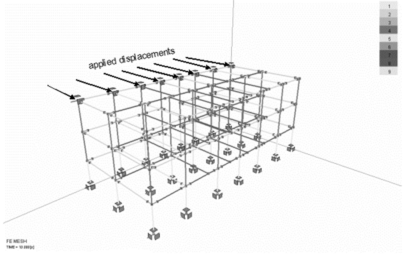
The nonlinear response of 2D equivalent & 3D model of an existing building under imposed displacement in the top is presented in this section before the pushover analysis. See Figure 6 and Figure 7 which represent the model in two figures for 2D equivalent & 3D models respectively.

This 2D equivalent model is obtained by making the sum of the stiffness, nodal masses and reinforcement of each frame but the longitudinal beams are neglected.

https://cdn.apub.kr/journalsite/sites/durabi/2021-012-01/N0300120101/images/Figure_susb_12_01_01_F6.jpg

Figure 6.

Equivalent 2D model under imposed displacement in the top.

https://cdn.apub.kr/journalsite/sites/durabi/2021-012-01/N0300120101/images/Figure_susb_12_01_01_F7.jpg

Figure 7.

3D model under imposed displacement in the top.

https://cdn.apub.kr/journalsite/sites/durabi/2021-012-01/N0300120101/images/Figure_susb_12_01_01_F8.jpg

Figure 8.

Comparison between 3D and equivalent 2D mode under imposed displacement in the top

Soil Structure 2D and 3D model using Lyzmer type viscous damper

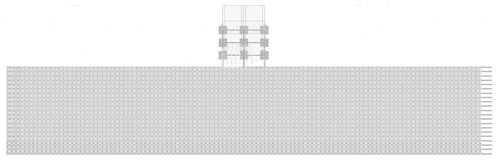
In this section, both 3D and 2D model of an existing structure are presented, taking into account the soil by introducing Lyzmer type viscous dampers, and the earthquake response see Figure 9 and Figure 11, respectively.

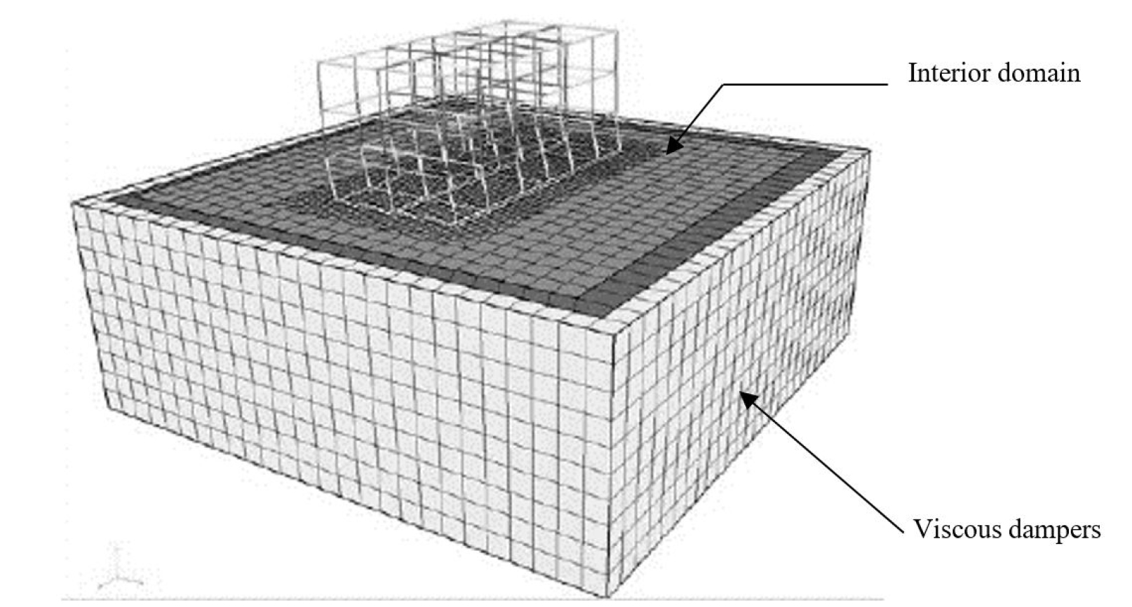
https://cdn.apub.kr/journalsite/sites/durabi/2021-012-01/N0300120101/images/Figure_susb_12_01_01_F9.jpg

Figure 9.

3D model of soil and structure using DRM and flexibility base method with Lyzmer damper [11].

https://cdn.apub.kr/journalsite/sites/durabi/2021-012-01/N0300120101/images/Figure_susb_12_01_01_F10.jpg

Figure 10.

Earthquake response of 3D model.

https://cdn.apub.kr/journalsite/sites/durabi/2021-012-01/N0300120101/images/Figure_susb_12_01_01_F11.jpg

Figure 11.

2D model of soil and structure.

https://cdn.apub.kr/journalsite/sites/durabi/2021-012-01/N0300120101/images/Figure_susb_12_01_01_F12.jpg

Figure 12.

Earthquake response of 2D model.

Results and discussion

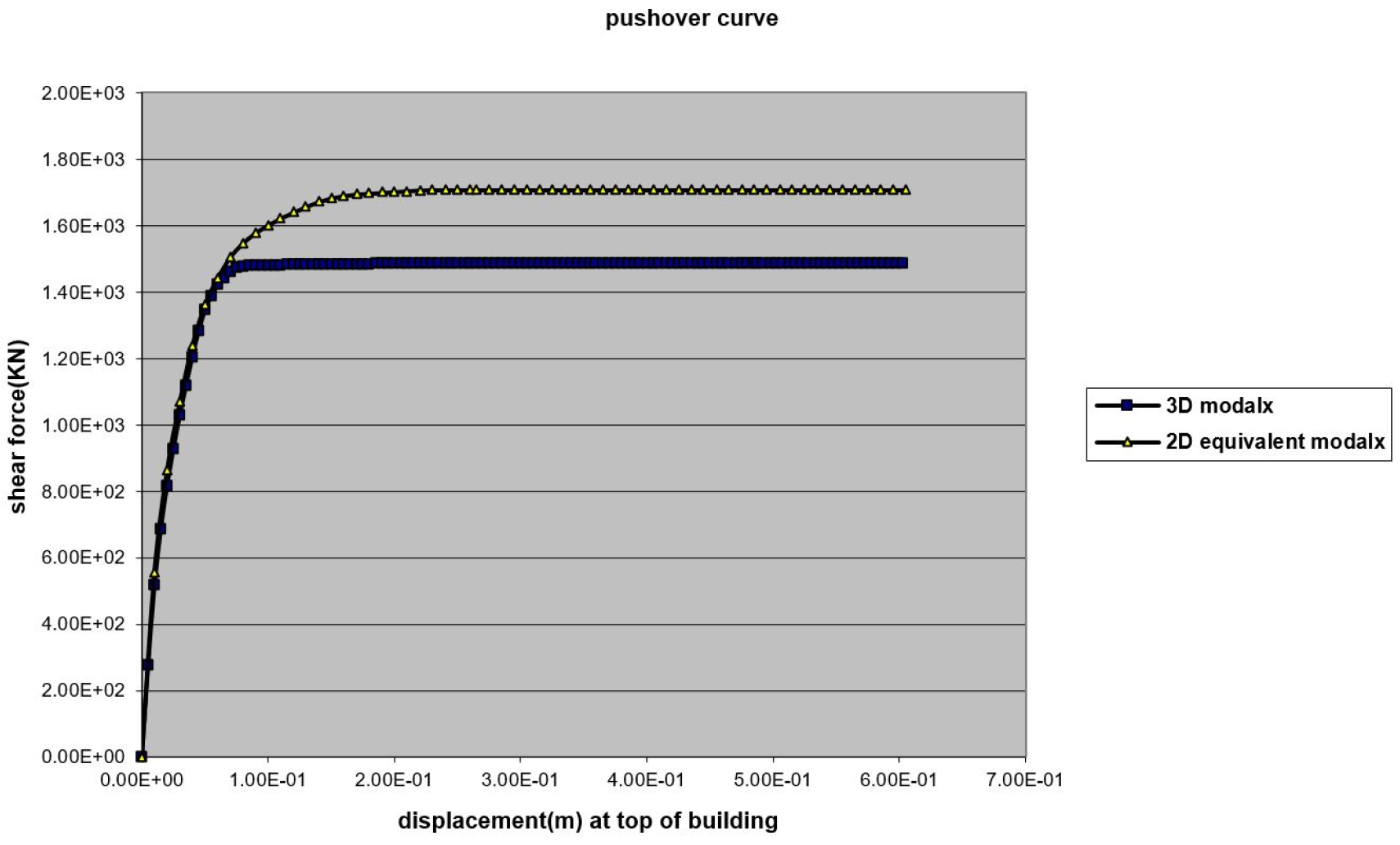
Figure 8 clearly shows the difference in results, between 3D & 2D equivalent model. There is no difference in the elastic state. In the first nonlinear state, a little difference between 2D equivalent & 3D model appear, but in the second nonlinear state this difference increase. Adeptly this is because the plastics hinges appear in different place between the two models.

At the top of the building indicate that 2D and 3D models are equivalent in the elastic range, then a stiffer behavior of the 2D model, moderate in the early nonlinear behavior, significant (20%) close to the maximum base shear. This seems to indicate a truly 3D resistance mode in the nonlinear range.

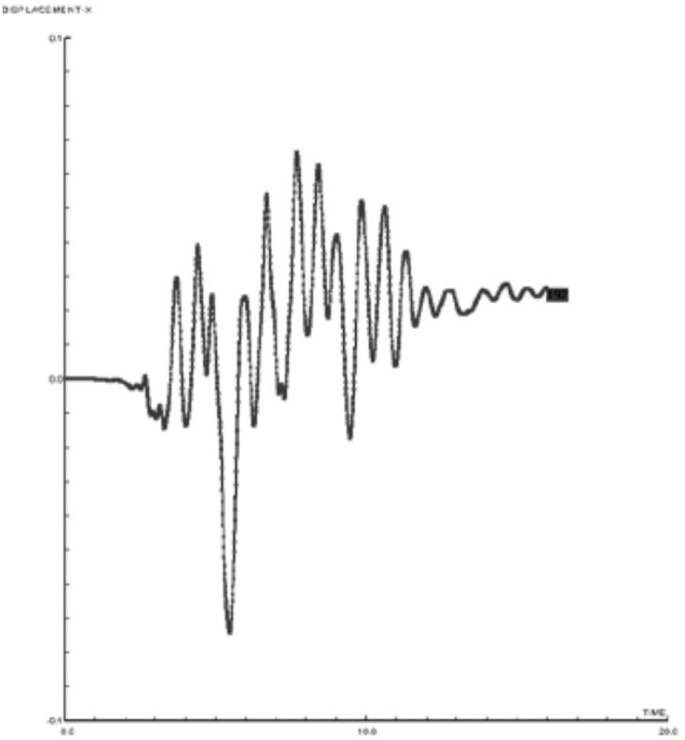
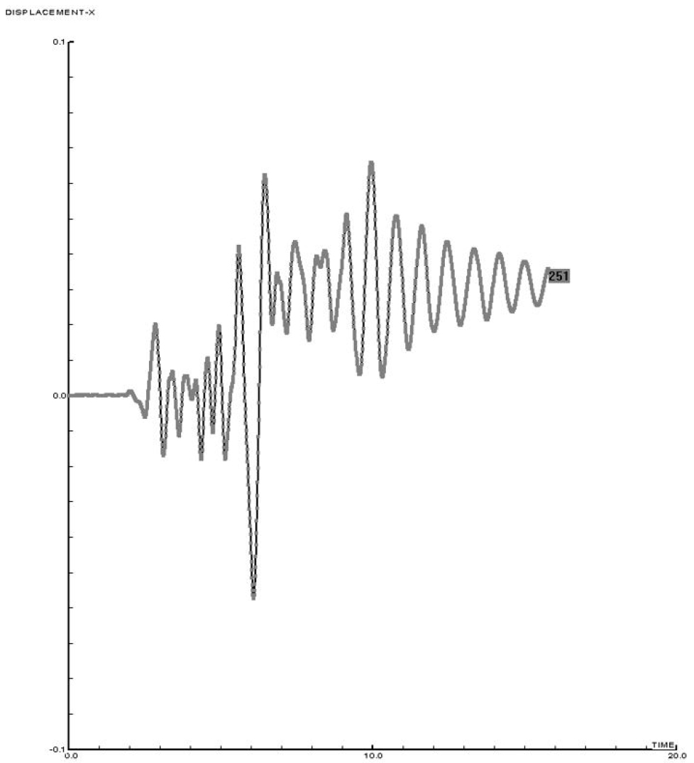
Figure 10 and Figure 12, show a clear difference between the maximum value of dynamic response, which are 0.07 m, and 0.063 m for 3D and 2D model, respectively. This difference appears even in the elastic stage.

Conclusion

The two methods (flexibility based model and domain reduced model) offers undeniable advantages namely the reduction of the size of the matrices that must be managed when the problem is solved. These elegant approach, allow to apprehend the actual behavior of the structure in a best manner. Thanks to domain reduction method who removes the fear of modeling the soil, which allows an optimization of soil modeling, at lower cost in terms of time and closer to reality. Especially by introducing Lyzmer type viscous dampers, which is one of the simplest ways to avoid reflections of waves outgoing from the domain. From Table 1 it is clear that the 2D and 3D models are very close in the case of uniform loading unlike modal loading this indicates the effect of the higher mode on the response. This shows the importance of 3D model because it allows to get as close as possible to reality. Without this type of model, the results tend to move away from the real behavior of the structure especially when this latter (behavior) enters a nonlinear phase.

Table 1.

Summary of pushover results for SDOF and MDOF system

Target displacements for	2D	3D
Uniform load single degree of freedom (SDOF)	0.051 m	0.052 m
Modal load single degree of freedom (SDOF)	0.042 m	0.06 m
Uniform load multi degree of freedom (MDOF)	0.0612 m	0.067 m
Modal load multi degree of freedom (MDOF)	0.0504	0.077 m

Solving a transient dynamic soil-structure interaction problems for single-phase media or two-phases media is possible now in a simple personal computer.

References

P. Fajfar, Capacity spectrum method based on inelastic demand spectra. Earthquake engineering and structural dynamics. 28 (1999), pp. 979-993. 10.1002/(SICI)1096-9845(199909)28:9<979::AID-EQE850>3.0.CO;2-1

A. Truty, Zimmermann Th. Dynamics in Z-SOIL, Z-SOIL PC. report Swiszerland. 2013.

J. Bielak, K. Loukakis, Y. Hisada, and C. Youshimura, DRM for 3D earthquake modeling in localized regions, part I: theory. Bulletin of the seismological society of America. 93 (2003), pp. 817-824. 10.1785/0120010251

M. Belgasmia, Optimization of Design for Better Structural Capacity. 2019, USA :IGI Global, ISBN: 9781522570592. 10.4018/978-1-5225-7059-2

E. Spacone, Flexibility-based finite element models for the nonlinear static and dynamic analysis of concrete frame structures. Dissertation, PhD Thesis, Department of Civil Engineering, University of California, Berkeley, 1994.

E. Spacone, F.C. Filippou, F.F. Taucer, Fiber beam column model for nonlinear analysis of R/C frames. I: Formulation, II: Applications. Earthquake Engineering and Structural Dynamics. 25(7) (1996), pp. 711-742. 10.1002/(SICI)1096-9845(199607)25:7<727::AID-EQE577>3.0.CO;2-O

M. Belgasmia and S. Moussaoui, Comparison between static nonlinear and time history analysis using flexibility Based Model for an existing Structure and Effect of taking into account soil using domain reduction method for a Single Media. KSCE Journal of Civil Engineering, 19(3) (2015), pp. 651-663. 10.1007/s12205-015-0351-y

T.J.R. Hughes, The finite element method : Linear Static and dynamic finite element analysis, 2000, Dover Publications INC Mineola New York.

M. Belgasmia, E. Spacone, and A. Urbanski, Zimmermann Th. Seismic evaluation of constructions : Static pushover procedure and time history analysis for nonlinear frames. LSC internal report, Swiss Federal Institute of Technology Lausanne Switzerland, 2007.

Eurocode 8. Design of structures for earthquake resistance, european committee for standardization, Part 1 General Rules. Seismic Actions and Rules for Buildings, 2003.

S. Command, Pushover analysis with Z-soil taking soil into account. Numerics in Geotechnics and Structures Symposium. 28 Years of Z-soil and Structure PC, Swiszerland, 2013.

International Journal of Sustainable Building Technology and Urban Development ISSN:2093-761X(Print) 2093-7628(Online)

Preview

Soil structure interaction using Lyzmer type viscous dampers and domain reduction method with flexibility-based model for an existing structure and comparison between 3D and 2D model without Soil modelization

ABSTRACT

MAIN

(1)

(2)

(3)

(4)

(5)

(6)

(7)

(8)

(9)

(10)

(11)

(12)

(13)

(14)

(15)

(16)

Figure 1.

Capacity curve: transformation from response of MDOF to equivalent SDOF.

Figure 2.

Bilinearization of the SDOF capacity curve.

Figure 3.

Foundation building plan.

Figure 4.

First and second floor building plan.

Figure 5

Third level and roof building plan.

Figure 6.

Equivalent 2D model under imposed displacement in the top.

Figure 7.

3D model under imposed displacement in the top.

Figure 8.

Comparison between 3D and equivalent 2D mode under imposed displacement in the top

Figure 9.

3D model of soil and structure using DRM and flexibility base method with Lyzmer damper [11].

Figure 10.

Earthquake response of 3D model.

Figure 11.

2D model of soil and structure.

Figure 12.

Earthquake response of 2D model.

Table 1.

Summary of pushover results for SDOF and MDOF system

References