Dual-path multi-scale attention guided network based changes in land use/land cover classification

Md. Arman Ali; Lalbahadur Roy

doi:10.22712/susb.20240030

Preview

General Article

International Journal of Sustainable Building Technology and Urban Development. 30 September 2024. 433-445
https://doi.org/10.22712/susb.20240030

Dual-path multi-scale attention guided network based changes in land use/land cover classification

Md. Arman Ali¹^*

Lalbahadur Roy²

¹Ph.D Student, Department of Civil Engineering, NIT Patna, Ashok Rajpath, Patna, Bihar, India

²Professor, Department of Civil Engineering, NIT Patna, Ashok Rajpath, Patna, Bihar- 800005, India

^{*Corresponding Author}

License (open-access, https://creativecommons.org/licenses/by-nc/4.0/):

This is an Open Access article distributed under the terms of the Creative Commons Attribution Non-Commercial License (https://creativecommons.org/licenses/by-nc/4.0/) which permits unrestricted non- commercial use, distribution, and reproduction in any medium, provided the original work is properly cited.

ABSTRACT

One of the most important environmental changes brought on by human activity is changes in land use and land cover (LULC), particularly in places that are quickly growing. In this manuscript proposes, Changes in Land Use and Land Cover Classification using a Dual-path Multi-scale Attention Guided network (LCC-DPAGN-LOA) is presented. This study utilizes data from the Remote Sensing dataset. Then pre-processing using Fast Resampled Iterative Filtering (FRIF) to enhance image quality. Feature selection is performed utilizing Quadratic Phase Wavelet Packet Transform, followed by classification using a DPAGN. After that the extracted features are provided to the Dual-path Multi-scale Attention Guided Network (DPAGN) is used for the classification of Agriculture, Bare lands, Built-up Areas, Forests and Water Bodies. In general, the DPAGN does not express adapting optimization techniques to determine optimal variables to ensure accurate classification. Therefore, it is proposed to utilize the Lyrebird Optimization Algorithm (LOA) to enhance DPAGN for accurate land cover classification. The proposed LCC-DPAGN-LOA technique is implemented in Python and analyzed performance metrics likes accuracy, recall and precision. The proposed method attains 20.78%, 17.98% and 25.67% higher accuracy than existing methods like Artificial Neural Network (ANN), Particle Swarm Optimization (PSO), and Elephant Herd Optimization (EHO) for land use and land cover classification respectively.

Keywords

land use/land cover changes

dual-path multi-scale attention guided network

fast resampled iterative filtering

quadratic phase wavelet packet transform

MAIN

Introduction
Literature Review
Proposed Methodology
Data Acquisition
Pre-processing using Fast Resampled Iterative Filtering
Feature Extraction using Quadratic Phase Wavelet Packet Transform (QPWPT)
Classification by Dual-path Multi-scale Attention Guided Network
Proposed Lyrebird Optimization Algorithm
Result and discussion
Discussion
Conclusion

Introduction

Land cover and usage changes in a region are the outcome of natural and socioeconomic forces interacting across time and space [1]. Changes in LULC are primarily impacted by changes in the system’s population growth rate, economic expansion, and physical characteristics including terrain, soil type, slope condition, and climate. The way that humans utilize the land has changed historically is a factor in land-use change [2]. Numerous resources, including water, soil, and vegetation, become less accessible. Evapotranspiration, groundwater penetration, and overland runoff are all immediately affected by changes in land use [3, 4]. Modifications to land cover and usage are significant issues when taking into account global dynamics and how they react to socioeconomic and environmental factors. Modifications to land cover and usage have an adverse impact on local and global socioeconomic dynamics, natural disasters, and climatic trends [5]. The classification of land cover, integral to urban planning, environmental management, agriculture, disaster response, and more, categorizes land into types like urban, forest, water, and agricultural areas [6]. It supports activities such as infrastructure development, crop monitoring, ecosystem assessment, disaster response planning, and city planning [7, 8]. In all industries, the combination of remote sensing and machine learning-based land cover categorization is crucial, providing critical information for informed decision-making and sustainable resource management [9]. The main problem that appears in existing approaches is firstly, the conversion of natural habitats into urban, agricultural, or industrial areas results in habitat loss and fragmentation, leading to a decline in biodiversity and ecosystem services [10]. Moreover, such changes can exacerbate climate change by reducing carbon sequestration capacity and altering local climate patterns. Additionally, intensive agricultural practices and urbanization often contribute to soil degradation, including erosion, compaction, and loss of fertility, which in turn impacts agricultural productivity and ecosystem health [11, 12]. These shortcomings of the current approach motivate us to conduct this study. The LCC-DPAGN-LOA system innovates by integrating enhanced feature extraction and employs a novel DPAGN for classification.

This work’s primary contribution is,

ㆍThe study utilizes data from the Remote sensing Dataset; it is frequently employed for classifying land cover and usage.

ㆍThe manuscript employs preprocessing technique Fast Resampled Iterative Filtering (FRIF) to improve the quality of the input images. Feature selection is performed using the Quadratic Phase Wavelet Packet Transform (QPWPT).

ㆍThe classification task is carried out using a DPAGN.

ㆍThe weight parameters of DPAGN are optimized with Lyrebird Optimization Algorithm.

This study is structured as: An overview of the relevant literature is given in Sector 2. Sector 3 outlines the proposed strategy, Sector 4 explains the results and a discussion, and Sector 5 concludes.

Literature Review

Numerous studies were previously submitted based on land cover classification a few works were reviewed here,

G.B. Rajendran et al., [13] have presented many land-use inventories and environment modeling depends heavily on the categorization of LULC using remote sensing data. To enhance the performance of LULC classification and aid in the prediction of animal habitat, declining environmental quality, haphazard components, etc., the suggested study presents a deep learning classifier and a hybrid feature optimization method. Two advantages of these hybrid optimizations are their great discriminative power and their invariance to grayscale and color images. To select the finest qualities, a human group-based PSO technique is then used. This approach has the advantages of a quick convergence rate and being simple to apply.

M. Kilany et al., [14] have presented an innovative strategy that combines the Random Forest (RF) classifier using the meta-heuristic optimization method known as Elephant Herding Optimization (EHO) algorithm, raising the precision of urban land cover categorization. The suggested method includes feature selection for a given urban area’s data collection in addition to classifier hyper parameter tweaking.

B. Sajan et al., [15] have presented the LULCC in District Muzaffarpur, the area in the Indian state of Bihar with the fastest-changing topography. This area is well-known for its litchi cultivation, which has been seen to be expanding in the area over the past several years in response to a decline in native vegetation. The goal of the suggested work was to assess the LULC of the Muzaffarpur district in the past, present, and future using support vector classification and CA-ANN techniques.

A kumar et al., [16] have presented the right location for the disposal of solid waste was crucial, as were many other considerations including social acceptability and sustainability. The suggested article aims to demonstrate the use of GIS in locating appropriate garbage disposal sites. It shows how land cover and usage were changing in the state of Bihar’s planned smart cities Bhagalpur, Patna, Muzaffarpur, and Biharsharif in a spatiotemporal manner. Major studies demonstrate the current situation of solid waste management in major cities in Bihar, even though a variety of variables, such as land use/cover, communication routes, and geomorphological changes, must be taken into consideration when selecting a location for the appropriate disposal of municipal solid waste.

M.Z. Hoque et al., [17] have presented the global LULC pattern and the ES it provides have undergone significant changes due to increased human activity and dynamic climatic factors. The impact of these LULC dynamics on natural resources, particularly in Bangladesh, hasn’t been thoroughly studied, nevertheless. Coastal Bangladesh: From 1999 to 2019, we assessed the dynamics of LULC change and related ecosystem service values (ESVs) using historical Landsat LULC images and economic valuation methods.

Proposed Methodology

In this section describes the DPAGN for accurate land cover classification. This study leverages the Remote Sensing Dataset and implements advanced techniques to improve land cover classification. The block diagram of the proposed LCC-DPAGN-LOA for accurate land cover classification is displayed in Figure 1. Consequently, the following provides a full description of LCC-DPAGN-LOA.

https://cdn.apub.kr/journalsite/sites/durabi/2024-015-03/N0300150309/images/Figure_susb_15_03_09_F1.jpg

Figure 1.

Block diagram of proposed Methodology LCC-DPAGN-LOA.

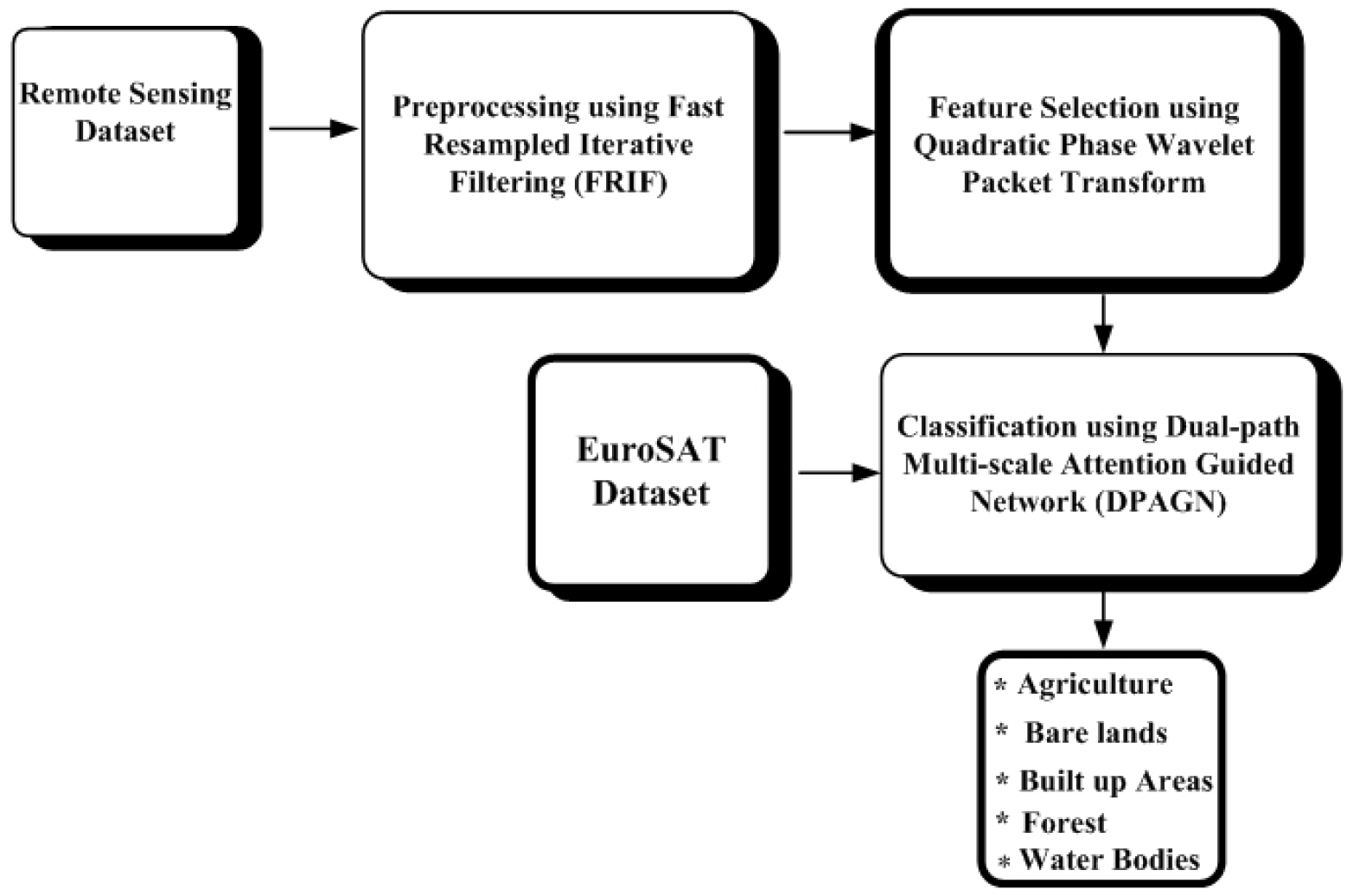
In the above block diagram the input images are collected from Remote Sensing Data. The input images are given to pre-processing by using fast resampled iterative filtering. Pre-processing aims to is to reduce the noise and sharpen the edges of images. The pre- processed image is given to quadratic phase wavelet packet transform for extracting the feature. The extracted features are given to DPAGN for accurate land cover classification of Agriculture, Bare lands, Built up Areas, Forests and Water Bodies. The weight parameter of DPAGN is optimized with Lyrebird Optimization Algorithm.

Data Acquisition

The data is collected from a satellite remote sensing dataset [18]. Prior to analysis and interpretation, the satellite photos underwent sorting and classification. One of the most popular types of satellite remote sensing data is Landsat imagery, which is helpful for mapping and planning projects due to its spectral, geographical, and temporal resolution. Land Use/Land Cover categories from LISS III images captured in 2005, 2011, and 2015 were used in this investigation. The coordinate systems of WGS-1984 and UTM Zone-45N are projected onto the photographs.

Pre-processing using Fast Resampled Iterative Filtering

In this step, image pre-processing using Fast Resampled Iterative Filtering (FRIF) [19] is discussed. The proposed FRIF has the aim to reduce the noise and sharpen the edges of images. Fast Resampled Iterative Filtering is intended to be a quick and efficient way of processing images, resulting in quicker processing times than previous filtering methods. This filter is intended to maintain the borders of objects in the picture, assuring that critical details are not lost during the pre-processing stage. By increasing the brightness of the images, the FRIF makes them easier to analyze and more visually attractive. It operates as continuously performing a set of filtering operations to the picture and reproducing them at each stage to reduce the amount of computing and improve performance. The Fast Resampled function is given in equation (1),

(1)

h_{n + 1} (H (y) \approx h_{n} (H (y)) - \int_{S} h_{n} (H (y)) l (y - z) d z

where, $h_{n + 1}$ represents pixel in image, $H (y)$ represents an integer, $h_{n}$ represents variable for removing the noise, $l$ represents filter weight, $l$ represents inverse of weight matrix and $d z$ represents the differentiation matrix. FRIF is especially beneficial when analysing big or high-resolution images, as typical approaches to filtering can be computationally costly. The recurring nature of the method allows for fine-tuning of filtering parameters to produce the best results. The quadrature rule is given in equation (2),

(2)

i_{n + 1} (y_{j}) \approx i_{n} (y_{j}) - \frac{N}{n} \sum i_{n} (y_{k}) l (y_{j} - y_{k})

where, $i_{n + 1} (y_{j})$ represents the quadrature rule, $n$ represents the parameter, $N$ represents the maximal window value, $i_{n}$ represents the feasible parameter, $y_{j}$ represents the covariance matrix, and integrated value $y_{k}$ represents size of images. The Hermitian circular matrix is given in equation (3),

(3)

i_{n + 1} = j f (1 - f (l_{1})) ‧ f (i_{n})

where, $l_{1}$ represents the Hermitian matrix, $l (0)$ represents the symmetrical shape of images, and $t$ represents the time-bandwidth. It makes it ideal for applications that work in real time that demand rapid picture processing. To determine an objective assessment of $i_{n + 1}$ , use balanced least squares estimation with the weighting matrix equal to the inverse of $f (i_{n})$ is given in equation (4),

(4)

i_{n + 1} = j f (1 - f (l_{1})) ‧ f (i_{n})

where, $j$ represents inverse matrix, $f$ represents the lighting, represents the product factor. In this case, the minimum time-bandwidth combination longer represents the area of the window. The deviation to the Fast Resampled Iterative Filtering curve may be removed, and the shortened window can be estimated to have the shortest time-bandwidth product if the discarded points are sufficiently tiny. The mathematical formula for the edge shaping is given in equation (5),

(5)

f (i_{n + 1}) = (1 - f (l_{1})) f (i_{n})

where, $f (i_{n + 1})$ represents the edge of the images, and ° represents the product matrix of fast resampled iterative. Thus reduce of noise and sharpen the edges of images from the image has been done by using the Fast Resampled Iterative Filtering method. Then, the pre-processed image is the feature extraction phase.

Feature Extraction using Quadratic Phase Wavelet Packet Transform (QPWPT)

In this step, Feature Extraction using QPWPT [20] is discussed. QPWPT is utilized to extract characteristics like uniformity and mean intensity. The quadratic phase wavelet packet transform represents the image more efficiently than typical wavelet transformations. It records the image’s magnitude and phase information, which allows a deeper examination of its characteristics. This means that the bulk of the images information is kept in a limited number of transform coefficients, resulting in much lower image storage needs and computational complexity during feature extraction. Quadratic Phase algorithm to estimate group delay is given in equation (6),

(6)

X_{g}^{η} (ϑ, α, φ) = \int_{s} g (u) L_{η} (u, ϑ)

where, $X_{g}^{η}$ represents the Quadratic Phase algorithm, 𝜗 represents frequency varying linear chirp signal, 𝛼 represents constant variables, 𝜑 represents the extracting relevant images, $g$ represents time reassignment operator, $u$ represents sequence of the scalar product, and $L_{η}$ represents the time axis of the ridge curve. It divides the image pixel for feature extraction. Reassignment operator of the image is given in equation (7),

(7)

X_{g}^{η} (ϑ, α, φ) = \int_{s} f^{j \cot y (u^{2 - α^{2}})} d u

where, $f$ represents the reassignment operator, $j$ represents the constant value, 𝛾 represents the impulsive value, and $d u$ represents the differentiation curve of the time axis. It integrates the ideas of wavelet transform with multi-resolution analysis. Time axis of the ridge curves is given in equation (8),

(8)

g_{ϑ η} = \sqrt{\frac{c}{2 Π j}} f^{j (b u^{2} + c u ϑ + d ϑ^{2})} g (u)

where, $g_{ϑ, η}$ represents the time axis curve, $c$ represents potential density, $b u$ represents the time varying of reconstruction of images, and $c u ϑ$ represents the combination of the potential density of the time ridge point. The QPWPT is given in equation (9),

(9)

R_{η} [g_{ϑ, n}] = \int L (x, u) g_{ϑ, n} (u) d u

Where, $R η$ represents wavelet transform function, $L$ represents first order features, and $x$ represents the total available features. In this transform the input image is synthesized in order to extract the image’s characteristics. The features such as mean intensity and uniformity were extracted.

Mean intensity: Mean intensity refers to the average intensity of grey numbers inside the pupil region. To compute the mean intensity, add all grey values in the pupil region and divide by the number of pixels which is given in equation (10),

(10)

n = \sum_{M - 0}^{M - 1} (\frac{J (u)}{o})

where, $n$ represents the average density, $J$ represents the possible intensity, $o$ signifies the number of pixel, and $M$ denotes the value of possible intensity level.

Uniformity: Uniformity measures the similarity of pixels in the pupil. Uniformity may be calculated by utilising the same grey value in a single region which is given in equation (11),

(11)

V = \sum_{M - 0}^{M - 1} {(\frac{I (0)}{o})}^{2}

where, $I$ represents the probability histogram, $O$ represents the count of pixels in the drawing area, $V$ represents the measure of the uniformity, and $M$ represents the value of possible intensity. The Quadratic Phase Wavelet Packet Transform was used to extract features like uniformity and mean intensity. These characteristics are then sent into the categorization stage.

Classification by Dual-path Multi-scale Attention Guided Network

In this section, classification and detection of neurodegenerative disease using DPAGN [21] is discussed. The DPAGN is a sophisticated deep learning architecture used for classification tasks, especially in the context of remote sensing and satellite imagery analysis. This type of network is well-suited for handling spatiotemporal data, making it particularly effective for classifying land cover types such as Agriculture, Bare lands, Built up Areas, Forest and Water Bodies. This mechanism allows the network to selectively attend to relevant temporal features at different time points, enhancing the model’s ability to capture temporal dynamics in land cover changes. Incorporate fusion techniques to combine information from multiple graphs representing criteria that different time instances. This fusion process ensures that the network leverages both past and present information for accurate classification. The graph convolution operation can be defined are given in equation (12)

(12)

B_{O, j k} = \{\begin{cases} 1, d i s (w j, w k) \leq M \\ 0, o t h e r w i s e \end{cases}

here, $B_{O, j k}$ represent the neighborhood graph, $w_{j}$ and $w_{k}$ are denotes the places and $M$ represent the graph Laplacian. Each item in the vector denotes number of points that belong to associated category and vector’s size is equal to number of functional categories. In a similar vein, it classifies the defected persons and it is given in equation (13),

(13)

B_{M, j, k} = s i m (T_{w_{j}}, T_{w_{k}}) \in [0, 1]

here, $B_{M, j, k}$ represent the defected persons and $T_{w_{j}}, T_{w_{k}}$ denotes the common symptom present in the defected persons $w_{j}$ and place $w_{k}$ respectively. This approach uses the created graph and multi-graph convolution to classify the satellite images of land cover,

(14)

Y_{m + 1} = \underset{B \in \bar{B}}{\cup} (σ f (B; θ_{j}) Y_{m} X_{m})

here, $Y_{m}$ and $Y_{m + 1}$ are represent the neurodegenerative diseases detection in layer $m$ and $m + 1$ , 𝜎 represent the variance in the symptoms, $\bar{B}$ represent the set of graph and $f (B; θ j)$ denotes the common symptoms based on graph. Equation (15) illustrates how graph convolution operation by max degree and related graph Laplacian matrix are used to classify the diseases.

(15)

{\overset{⏜}{Y}}^{(u)} = ⌊ Y^{(u)}, G_{H}^{L'} (Y^{(u)}) ⌋ u = 1, 2, . . . . U

here, $Y^{(u)}$ denotes the $t^{t h}$ observation to categorize land and cover images, $G_{H}^{L'}$ represents graph convolution for Agriculture, Bare lands, Built up Areas, Forest and Water Bodies, $L'$ specifies the extraction of the images and $U$ specifies the classifies. Thus, it classifies the diseases into five categories. It is given in equation (16),

(16)

a^{(u)} = G_{p o o l} ({\hat{Y}}^{(u)}) = \frac{1}{| W |} \sum_{u = 1}^{| W |} {\hat{Y}}_{j, :}^{(u)} u = 1, 2, \dots U

here, $a$ represent the input, ${\overset{⏜}{Y}}_{j, :}^{(u)}$ signifies $t^{t h}$ observation, $G_{p o o l}$ and represents classification of images. Equation (17), which applies to classify the satellite images,

(17)

t = σ (X_{2} δ (X_{1} a))

here, $X_{1}$ and $X_{2}$ are denotes the trainable weights, 𝛿 represent the classification of the images, 𝜎 denotes the reduction in spatial dimension and $t$ denotes the reweighting factor of bandwidth. Lastly, in equation (18) the reweighting factor is applied to the original historical input.

(18)

{\bar{Y}}^{(u)} = Y^{(u)} ° t^{(u)}

here ° denotes the dot product, $u$ denotes feature vector detection using a common CNN layer with weight across all regions after contextual gating it is shown in equation (19),

(19)

\begin{array}{r} I_{j, :}^{Q H} = DPAGN ({\bar{Y}}_{j, :}^{(u^{'})}, {\bar{Y}}_{j, :}^{(u^{'} + q)}, {\bar{Y}}_{j, :}^{(u^{'} + 2 q)} \\ \dots, {\bar{Y}}_{j, :}^{(U - q)}, {\bar{Y}}_{j, :}^{(U)}; X_{4}) \end{array},

here, $I_{j, :}^{Q H}$ represents the weight matrix, $q$ represent the training models, $q$ represent the periodic interval, depending on the features of the data. DPAGN represents a sophisticated neural network architecture that leverages advanced techniques in temporal data processing, graph convolution, and gated mechanisms to address the challenges inherent in land cover classification such as Agriculture, Bare lands, Built up Areas, Forest and Water Bodies. In this work, LOA for accurate land cover classification in deep learning, this method optimizes the DPAGN optimum parameter $w_{α} a n d w_{β}$ . Here, LOA is applied for tuning the weight and bias parameters of DPAGN.

Proposed Lyrebird Optimization Algorithm

The weight parameter $w_{α} a n d w_{β}$ of DPAGN is optimized using the proposed LOA [22]. This section presents a novel bio-inspired metaheuristic algorithm known as the Lyrebird Optimization Algorithm (LOA), which mimics the behavior of lyrebirds in the wild. The lyrebird, one of the most well-known native birds of Australia, is identified by its unusual plumes of neutral-colored tail feathers. The proposed LOA technique, which is covered below, was created using mathematical modeling of this lyrebird tactic in times of peril.

Stepwise Procedure of LOA

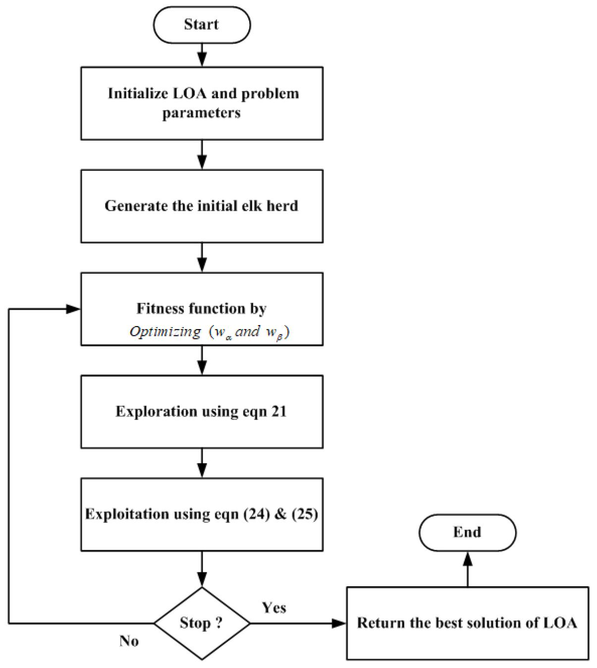
A step-by-step process is outlined here to determine the optimal DPAGN value depending on LOA. To maximize the DPAGN parameter, LOA first creates an evenly distributed population. Using the LOA algorithm, the best solution is promoted and related flowchart is illustrated in Figure 2.

https://cdn.apub.kr/journalsite/sites/durabi/2024-015-03/N0300150309/images/Figure_susb_15_03_09_F2.jpg

Figure 2.

Flowchart of LOA.

Step 1: Initialization

Initially, randomness generates the LOA population. Then the initialization is derived in equation (20),

(20)

B = [\begin{array}{cccc} b_{1}^{1} & b_{2}^{1} & \dots & b_{N}^{1} \\ b_{1}^{2} & b_{2}^{2} & \dots & b_{N}^{2} \\ ⋮ & ⋮ & \dots & ⋮ \\ b_{1}^{e h s} & b_{2}^{e h s} & \dots & b_{N}^{e h s} \end{array}]

where, $B$ are denoted as Lyrebird; $N$ is the total amount of characteristics or solution dimensionality in each LOA solution and $b$ establishes the feathers of LOA.

Step 2: Random Generation

After initialization, the input’s factors are generated at random. The optimal fitness value to select is determined by their explicit hyper parameter condition.

Step 3: Fitness Function

An arbitrary solution is produced by using initialized evaluations. Evaluation of fitness values makes use of the weight parameter $w_{α} a n d w_{β}$ it given in equation (21)

(21)

F i t n e s s f u n c t i o n = O p t i m i z i n g (w_{α} a n d w_{β})

Step 4: Escaping Strategy (Exploration Phase)

In this stage of LOA, the population member’s position in the search space is updated using a model that simulates the lyrebird’s departure from the risk position to the safe zones. When the lyrebird is moved to a secure environment, it undergoes significant positional changes and searches various regions of the problem-solving space, demonstrating LOA’s capacity for global search exploration. According to the LOA design, other population members with greater objective function values are positioned in a member’s safe regions. Equation (22) can therefore be used to determine the set of safe zones for every member of the LOA.

(22)

D B_{j} = {Z_{P}, E_{P} < E_{j} a n d P \in {1, 2, . . . . ., M}}, W h e r e j = 1, 2, . . . . . . . . ., M,

here $D B_{j}$ is indicated as the group of places where the jth Lyrebird is safe and $Z_{P}$ is represented as the Z matrix’s Pth row, which is superior than the jth LOA component in terms of objective function value

The LOA design allows for the possibility that the lyrebird will occasionally find its way to one of these safe havens. Equation (23) is used to compute a novel location for every LOA member based on the displacement modeling of lyrebirds carried out in this phase. Next, in accordance with Equation (24), this novel location replaces the place of the linked member’s previous location if the value of the goal function is increased.

(23)

z_{j, i}^{k 1} = z_{j, i} + l_{j, i} . (S S B_{j, i} - J_{j, i} . z_{j, i})

(24)

Z_{j} = \{\begin{cases} Z_{j}^{k 1}, E_{j}^{k 1} \leq E_{j} \\ Z_{j}, Else \end{cases}

here, $S S B_{j, i}$ is represented as its ith dimension, $S S B_{j}$ is indicated as the region designated as safe for ith Lyrebird, $z_{j}^{k 1}$ is denoted as the new location determined for the jth lyrebird using the proposed LOA’s escape plan, $z_{j, i}^{k 1}$ is represented as its ith dimension, $E_{j}^{k 1}$ is denoted as its objective function value, $l_{j, i}$ are represented as random values inside the range [0, 1], and $J_{j, i}$ are indicated as integers that are chosen at random to be either 1 or 2.

Step 5: Exploitation Phase for optimizing 𝜃

The population member’s position is updated in the search space throughout this stage of LOA based on the lyrebird’s modeling technique for hiding in its local safe zone. The lyrebird uses LOA in local search because it keeps a close eye on its surroundings and makes small movements to go to a decent hiding site, which causes its position to vary somewhat. Equation (25), which models the lyrebird’s migration to the nearest suitable hiding place, is employed in LOA design to determine each LOA member’s new position. This new location replaces the former position of the relevant component if, according to Equation (26), it raises the value of the goal function.

(25)

z_{j, i}^{k 2} = z_{j, i} + (1 - 2 l_{j, i}) . \frac{v c_{i} - q c_{i}}{T}

(26)

Z_{j} = \{\begin{cases} Z_{j}^{k 2}, E_{j}^{k 2} \leq E_{j} \\ Z_{j}, Else \end{cases}

here, $z_{j}^{k 2}$ is indicated as the jth Lyrebird’s new position as determined by the proposed LOA’s hiding method, $z_{j, i}^{k 2}$ is denoted as its ith dimension, $l_{j, i}$ are indicated as random values inside the range [0, 1], $E_{j}^{k 2}$ is represented as its objective function value, and $T$ is denoted as the iteration counter.

Step 6: Termination Criteria

If the termination requirement is met, the finest solution has been discovered; if not, carry out the previous steps again.

Result and discussion

The proposed technique LCC-DPAGN-LOA is implemented in Python and analyzed performance metrics likes accuracy, precision and recall. The proposed method LCC-DPAGN-LOA is compared with existing methods like LCC-PSO, LCC-EHO and LCC-ANN respectively.

ㆍTP:True positive occurs when classification method correctly forecasts positive class as positive.

ㆍTN:True negative occurs when classification method correctly forecasts negative class as negative.

ㆍFP:False positive occurs when classification method incorrectly forecasts negative class as positive

ㆍFN:False negative occurs when classification method incorrectly forecasts positive class as negative.

Accuracy: The ratio of properly categorized examples to total occurrences is utilized to determine accuracy that gauges how accurate the model’s predictions are overall. It is calculated by equation (27),

(27)

Accuracy = \frac{T P + T N}{Total Ins tan ces}

Precision: Precision is used to gauge how well the model predicts the favorable outcomes. The ratio is calculated between all actual positive cases and all projected positive cases. It is calculated by equation (28),

(28)

P r e c i s i o n = \frac{T P}{T P + F P}

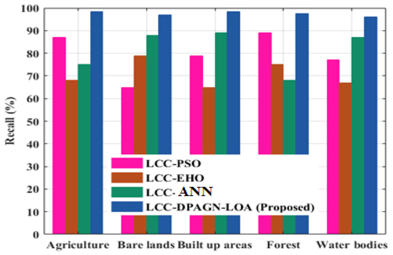
Recall (Sensitivity): The model’s recall quantifies how well it can recognize positive examples. The ratio of genuine positive instances to all actual positive instances is computed. It is calculated by equation (29),

(29)

R e c a l l = \frac{T P}{T P + F N}

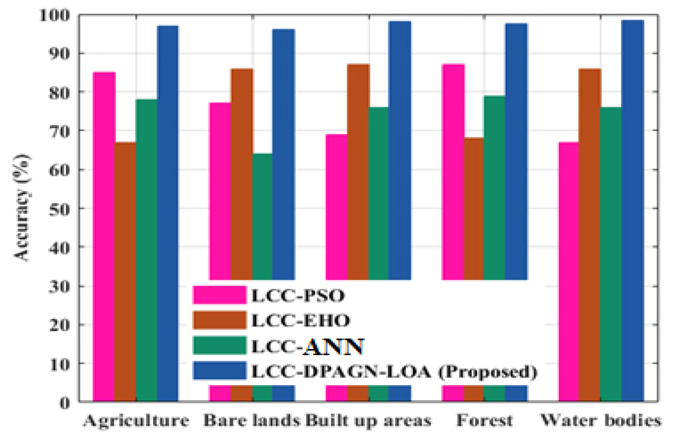
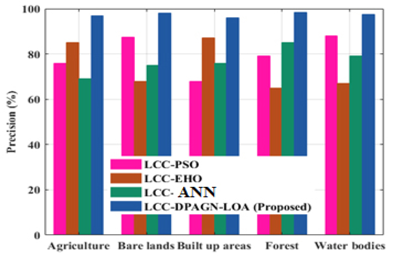
Figure 3 shows accuracy analyses. The performance of LCC-DPAGN-LOA technique results in accuracy that are 30.76%, 25.97%, and 24.67% higher for the classification of agriculture, 25.58%, 23.64% 38.783% higher for the classification of Bare land, 20.76%, 28.43% and 25.89% higher for the classification of built up area, 33.76%, 34.97%, and 12.67% higher for the classification of forest, 15.58%, 33.64% and 37.783% higher for the classification of water bodies when evaluated to the existing LCC-PSO, LCC-EHO and LCC-ANN methods. Figure 4 portrays precision analyses. The LCC-DPAGN-LOA technique results in precision that are 30.66%, 22.97%, and 25.67% higher for the classification of agriculture, 35.58%, 33.64% and28.783% higher for the classification of Bare land, 20.76%, 28.43% and 25.89% higher for the classification of built up area, 32.76%, 34.97%, and 12.67% higher for the classification of forest, 25.58%, 33.64% and 37.783% higher for the classification of water bodies when evaluated to the LCC-PSO, LCC-EHO and LCC-ANN methods. Figure 5 portrays recall analyses. The LCC-DPAGN-LOA technique results in recall that are 30.96%, 32.97%, and 25.87% higher for the classification of agriculture, 33.58%, 36.64% and 28.78% higher for the classification of Bare land, 20.76%, 28.43% and 25.89% higher for the classification of built up area, 22.76%, 24.97%, and 12.67% higher for the classification of forest, 35.58%, 33.64% and 37.783% higher for the classification of water bodies, when evaluated to the existing LCC-PSO, LCC-EHO and LCC-ANN methods respectively.

https://cdn.apub.kr/journalsite/sites/durabi/2024-015-03/N0300150309/images/Figure_susb_15_03_09_F3.jpg

Figure 3.

Accuracy analyses.

https://cdn.apub.kr/journalsite/sites/durabi/2024-015-03/N0300150309/images/Figure_susb_15_03_09_F4.jpg

Figure 4.

Precision analyses.

https://cdn.apub.kr/journalsite/sites/durabi/2024-015-03/N0300150309/images/Figure_susb_15_03_09_F5.jpg

Figure 5.

Recall analyses.

Discussion

The LULC Classification using Dual-path Multi-scale Attention Guided network addresses the critical need for accurate and efficient classification of LULC utilizing advanced deep learning techniques. The enhanced method’s performance is assessed utilizing standard metrics likes accuracy, precision, recall. Comparisons with previous approaches may also be included to demonstrate the improvement achieved through optimization. The proposed method LCC-DPAGN-LOA is compared with existing methods like LCC-PSO, LCC-EHO and LCC-ANN with higher accuracy.

Conclusion

The study on “LULC Classification using Dual-path Multi-scale Attention Guided Network” introduces a novel approach leveraging advanced deep learning techniques for improved land cover classification. By optimizing the Dual-path Attention Guided Network (DPAGN) with the Lyrebird Optimization Algorithm (LOA), substantial enhancements in classification performance were achieved. The LCC-DPAGN-LOA method outperformed traditional techniques, showing accuracy improvements of up to 38.78%, precision gains of up to 37.78%, and recall increases of up to 32.97% compared to methods such as LCC-PSO, LCC-EHO, and LCC-ANN. These improvements demonstrate the method’s effectiveness in capturing complex spatiotemporal patterns and spatial dependencies within satellite imagery. Enhanced classification accuracy contributes to more reliable environmental monitoring, better resource management, and improved urban planning. Despite these advancements, the study acknowledges limitations related to data variability, atmospheric conditions, and external factors like government policies and socioeconomic conditions. Future research should focus on increasing image quality, incorporating a broader range of socioeconomic and physical variables, and exploring hybrid models to further enhance performance. By addressing these issues, the fields of remote sensing and machine learning will improve and more accurate land cover mapping will be supported.

References

K.J. Gohain, P. Mohammad, and A. Goswami, Assessing the impact of land use land cover changes on land surface temperature over Pune city, India. Quaternary International. 575 (2021), pp. 259-269.

10.1016/j.quaint.2020.04.052

S. Thakur, D. Maity, I. Mondal, G. Basumatary, P.B. Ghosh, P. Das, and T.K. De, Assessment of changes in land use, land cover, and land surface temperature in the mangrove forest of Sundarbans, northeast coast of India. Environment, Development and Sustainability. 23 (2021), pp. 1917-1943.

10.1007/s10668-020-00656-7

B.M. Hashim, A. Al Maliki, M.A. Sultan, S. Shahid, and Z.M. Yaseen, Effect of land use land cover changes on land surface temperature during 1984-2020: A case study of Baghdad city using landsat image. Natural Hazards. 112(2) (2022), pp. 1223-1246.

10.1007/s11069-022-05224-y

N.N. Dey, A. Al Rakib, A.A. Kafy, and V. Raikwar, Geospatial modelling of changes in land use/land cover dynamics using Multi-layer Perceptron Markov chain model in Rajshahi City, Bangladesh. Environmental Challenges. 4 (2021), 100148.

10.1016/j.envc.2021.100148

A. Fayaz, M.U. Shafiq, H. Singh, and P. Ahmed, Assessment of spatiotemporal changes in land use/land cover of North Kashmir Himalayas from 1992 to 2018. Modeling Earth Systems and Environment. 6 (2020), pp. 1189-1200.

10.1007/s40808-020-00750-9

M.H. Edan, R.M. Maarouf, and J. Hasson, Predicting the impacts of land use/land cover change on land surface temperature using remote sensing approach in Al Kut, Iraq. Physics and Chemistry of the Earth, Parts A/B/C. 123 (2021), 103012.

10.1016/j.pce.2021.103012

P. Kumar, M. Dobriyal, A. Kale, and A.K.Pandey, Temporal dynamics change of land use/land cover in Jhansi district of Uttar Pradesh over past 20 years using LANDSAT TM, ETM+ and OLI sensors. Remote Sensing Applications: Society and Environment. 23 (2021), 100579.

10.1016/j.rsase.2021.100579

S.C. Sam and G. Balasubramanian, Spatiotemporal detection of land use/land cover changes and land surface temperature using Landsat and MODIS data across the coastal Kanyakumari district, India. Geodesy and Geodynamics. 14(2) (2023), pp. 172-181.

10.1016/j.geog.2022.09.002

H.B. Akdeniz, N.S. Sag, and S. Inam, Analysis of land use/land cover changes and prediction of future changes with land change modeler: Case of Belek, Turkey. Environmental Monitoring and Assessment. 195(1) (2023), 135.

10.1007/s10661-022-10746-w

S. Saumya and K. Rashmi, Analysis of land cover change and urban heat islands of Lucknow, India. International Journal of Sustainable Building Technology and Urban Development. 14(2) (2023), pp. 215-228.

G. Kalaimani, G. Kavitha, S. Chinnaiyan, and S. Mylapalli, Optimally configured generative adversarial networks to distinguish real and AI-generated human faces. Signal, Image and Video Processing. (2024), pp.1-18.

10.21203/rs.3.rs-4107900/v1

P. Rajesh, C. Naveen, A.K. Venkatesan, and F.H. Shajin, An optimization technique for battery energy storage with wind turbine generator integration in unbalanced radial distribution network. Journal of Energy Storage, 43 (2021), 103160.

10.1016/j.est.2021.103160

G.B. Rajendran, U.M. Kumarasamy, C. Zarro, P.B. Divakarachari, and S.L. Ullo, Land-use and land-cover classification using a human group-based particle swarm optimization algorithm with an LSTM Classifier on hybrid pre-processing remote-sensing images. Remote Sensing. 12(24) (2020), 4135.

10.3390/rs12244135

M. Kilany, C. Zhang, and W. Li, Optimization of urban land cover classification using an improved Elephant Herding Optimization algorithm and random forest classifier. International Journal of Remote Sensing. 42(15) (2021), pp. 5741-5763.

10.1080/01431161.2021.1931533

B. Sajan, V.N. Mishra, S. Kanga, G. Meraj, S.K. Singh, and P. Kumar, Cellular automata-based artificial neural network model for assessing past, present, and future land use/land cover dynamics. Agronomy. 12(11) (2022), 2772.

10.3390/agronomy12112772

A. Kumar, E. Singh, R. Mishra, and S. Kumar, Monitoring of land use/land cover changes by the application of GIS for disposal of solid waste: a case study of proposed smart cities in Bihar. InSustainability in Environmental Engineering and Science: Select Proceedings of SEES (2021) (pp. 253-262). Springer Singapore.

10.1007/978-981-15-6887-9_28

M.Z. Hoque, I. Islam, M. Ahmed, S.S. Hasan, and F.A. Prodhan, Spatio-temporal changes of land use land cover and ecosystem service values in coastal Bangladesh. The Egyptian Journal of Remote Sensing and Space Science. 25(1) (2022), pp. 173-180.

10.1016/j.ejrs.2022.01.008

S. Dutta, R.K. Ranjan, and A. Prakash, An Assessment of Land Use and Land Cover Change in Populous Districts of Bihar using Remote Sensing Database from Amity School of Earth & Environmental Sciences, Amity University, Haryana, published in Journal of Energy Research and Environmental Technology (JERET). p-ISSN: 2394-1561; e-ISSN: 2394-157X. 7(1) (2020), pp. 26-31.

M.Y. Bhat, A.H. Dar, D. Urynbassarova, and A. Urynbassarova, Quadratic-phase wave packet transform. Optik. 261 (2022), 169120.

10.1016/j.ijleo.2022.169120

Q. Ji, J. Wang, C. Ding, Y. Wang, W. Zhou, Z. Liu, and C. Yang, DMAGNet: Dual‐path multi‐scale attention guided network for medical image segmentation. IET Image Processing. 17(13) (2023), pp. 3631-3644.

10.1049/ipr2.12904

G. Barbarino and A. Cicone, Stabilization and variations to the adaptive local iterative filtering algorithm: The fast resampled iterative filtering method. Numerische Mathematik. 156 (2024), pp. 395-433.

10.1007/s00211-024-01394-y

M. Dehghani, G. Bektemyssova, Z. Montazeri, G. Shaikemelev, O.P. Malik, and G. Dhiman, Lyrebird optimization algorithm: a new bio-inspired metaheuristic algorithm for solving optimization problems. Biomimetics. 8(6) (2023), 507.

10.3390/biomimetics8060507

International Journal of Sustainable Building Technology and Urban Development ISSN:2093-761X(Print) 2093-7628(Online)

Preview

Dual-path multi-scale attention guided network based changes in land use/land cover classification

ABSTRACT

MAIN

Figure 1.

Block diagram of proposed Methodology LCC-DPAGN-LOA.

(1)

(2)

(3)

(4)

(5)

(6)

(7)

(8)

(9)

(10)

(11)

(12)

(13)

(14)

(15)

(16)

(17)

(18)

(19)

Figure 2.

Flowchart of LOA.

(20)

(21)

(22)

(23)

(24)

(25)

(26)

(27)

(28)

(29)

Figure 3.

Accuracy analyses.

Figure 4.

Precision analyses.

Figure 5.

Recall analyses.

References