Introduction

Excellent performance is required in all buildings to ensure protection and safety among people who reside and operate within them. In particularly, the performance of residential buildings is very important because people spend a considerable amount of time in a building. However, the performance of a building degrades over time [1], and this deterioration can take many forms.

A building façade, which is one of the important elements of a building, plays a role in preventing elements occurring in the external environment from affecting the building decoration, structural safety, insulation, comfort [2, 3]. Compared to the other elements of buildings, aging tends to rapidly progress because buildings are exposed to the external environment over a prolonged period. Rapid deterioration can appear as a defect, which can negatively affect façades (e.g., lowering the insulation effect of the building) [4]. However, it is impractical to prevent all the defects from occurring on the façades of a building in the pre-built stage. Therefore, it is important to detect and cope with such defects efficiently.

Existing defect management methods are mostly centered on manpower [5]. Accordingly, these methods are inefficient in terms of labor cost and time consumption and may cause life-threatening accidents [6]. In addition, because the results of an inspection can be subjective, it is necessary to inspect defects efficiently by minimizing the dependence on manpower through automated inspection technology.

Several types of defects occur on building façades depending on, for instance, humidity and façade type, and the sizes of such defects also vary [2]. In addition, there are also various types of non-defective objects such as windows, railings, and exhaust pipes. Because building façades and the defects occurring therein have the above characteristics, an automated defect detection system must be able to simultaneously detect and effectively classify various types of large and small defects using images of building façades with a complex background. Furthermore, if such a defect detection can be performed at high speeds, then defects may be simultaneously detected with the image captures of building façades. Through such a high-speed detection system, it is possible to efficiently manage defects in time, and accordingly, convenience and cost reduction can be expected.

Lee et al. (2020) [7] detected several types of defects using a model based on a deep convolutional neural network (DCNN) used in an object detection task, which is one of the major problems of deep learning. Lee et al. (2020) [7] aimed to maximize the detection performance and used a heavy model structure. The purpose of this study is to build a high-speed detection system for defects by reducing the inference time and the weight based on the heavy model. If a simple weight reduction is performed, then there is a high possibility that performance will be degraded depending on the characteristics of deep learning. Accordingly, this study aims to follow the detection performance of the existing model using a method to prevent performance degradation that occurs in the model compression process.

In this study, a deep learning model was used as a system to detect various types of defects occurring on building façades, and a knowledge distillation (KD) technique was used to speed it up and prevent performance degradation. The deep learning technique is a data-based method that does not require manual data collection or input. Building a deep learning model includes the process of selecting an appropriate model optimization algorithm and a loss function suitable for the model’s network structure and purpose.

The steps of this study are as follows: First, image data were collected to train a deep learning model. The data are image data of a façade of a residential facility collected using drones, and because the façade of a residential building is designed in various ways, it has a complex background. Subsequently, ground-truth boxes for various types of defects existing in these images and their class information were generated. Then, we selected a model for simultaneously detecting several types of defects and classifying them. The model was selected in consideration of the characteristics of the image data used in this study, and the faster region proposal convolutional neural network (Faster R-CNN) model was used as a basic model for training and evaluation. Because the goal of this study is to speed up the model, the basic model was lightened. However, lightened deep learning models tends to degrade the performance of the model. Therefore, we utilize KD techniques to prevent the phenomenon.

Literature Review

Prior research and limitations related to building maintenance

As mentioned in the Introduction section, because the performance of buildings deteriorates due to various factors, it is important to constantly check for various types of defects. Accordingly, several studies have been conducted to determine efficient building inspection methods [8, 9, 10]. Kim et al. (2013) [8] proposed a probabilistic framework for the maintenance plan and optimal inspection of structures with deteriorating conditions. Santos et al. (2017) [9] proposed a support system to standardize and systematize procedures for the inspection, diagnosis, and reconstruction of door and window frames. Bortolini and Forcada (2020) [10] proposed a Bayesian network approach to develop models for assessing the building condition. Most of these studies consider inspection strategies and maintenance plans. However, as mentioned in the Introduction section, manpower-based inspection has limitations, so it is necessary to develop a technology that can continuously and automatically monitor defects in buildings.

Accordingly, several studies have proposed the structural health monitoring (SHM) technique. In general, the SHM system utilizes a vibration-based structural system identification technique using a numerical method [11, 12, 13, 14]. However, the SHM system also has various limitations, such as compensation for cost issues and environmental impacts due to the installation of multiple sensors. Moreover, because it only monitors structural damage, it cannot detect various types of defects, such as cracks, leak marks, and corrosion.

To compensate for these problems, studies were conducted on defect detection methods based on image processing techniques [15, 16, 17]. In image processing technology, prior knowledge about images is used, and because images acquired in real life are very diverse, the recognition of defects existing in real images is limited [18].

Prior research on flaw detection using deep learning

In the field of image recognition with deep learning, image data-based learning is performed; thus, prior knowledge of images is not required. Accordingly, many studies have utilized deep learning to monitor defects in civil structures in the construction field and solve problems encountered in image processing technology. Previous studies have used deep learning techniques to detect cracks in various structures, particularly in sewage pipes [6, 19, 20]. Wang et al. (2020) [19] used CCTV image data as input data and combined a CNN and a conditional random field to detect three types of defects in drainage pipes. Zhang et al. (2019) [6] proposed a fully convolutional network based on a dilated convolution consisting of an encoder and a decoder for concrete crack detection. Wang et al. (2021) [20] proposed a framework based on defect detection and metric learning for tracking multiple defects of sewers using CCTV videos. Existing studies have focused on civil engineering structures, but such structures differ in buildings and facilities. Because the building façade is composed of various shapes, it is relatively important to recognize a specific defect in image data. In addition, the types of defects on the façade are diverse and the shape of defects is not regular. Thus, a model that can precisely detect and classify several types of defects at once is needed. Accordingly, Lee et al. (2020) detected various types of defects on the building façade using Faster R-CNN. Because this model aims to increase the accuracy of complex defect detection, the number of variables and operations in the model is large, and the inference time for new data is long. Therefore, to simultaneously perform defect detection and image collection, a technique to reduce the inference time using a lightweight model is required.

Prior research on high-speed detection models based on deep learning

Deep learning-based networks pass input data through several layers, extract features of the data, and learn based on the findings of the previous steps. Typically, when there is enough input data, if the deeper the layer of the network, then the higher the level of features that can be extracted, which improves the performance of deep learning model. That is, the performance of a network with a relatively shallow layer is lower than that of a network with a deep layer. However, a network with a deep layer has a large computational cost because it contains numerous parameters and computational processes. As a result, the inference time required to calculate the model’s output using the validation data increases. To compensate for these constraints, weight reduction can shorten the inference time of the model, but the performance of the model is degraded. To address this performance degradation, several studies have been conducted, aiming to mimic the performance of a network with a lightweight model but with a deep-layer model’s performance [21, 22, 23]. In the study of Hinton et al. (2015) [21], after learning a deep-layer network for a dataset of an image classification problem, a deactivated logit was extracted from the output layer of the network. Romero et al. (2015) [22] proposed using not only the logit of the output layer but also the output of the hidden layer for the learning of shallow networks. Chen et al. (2017) [23] evaluated the performance of the KD learning method by applying the above learning methods to the object detection task rather than simply classifying images. In the present study, we propose a method of distilling the knowledge of the deep-layered network into a shallow-layered network while using this knowledge to learn a relatively shallow-layer network.

Methodology

As described in the previous section, it is necessary to automate the detection of defects on the building façade for building maintenance, and it has been effective to utilize deep learning as an automation method. Therefore, in this work, we propose to check buildings based on deep learning models, and furthermore, we aim to use the model compression technique of deep learning models to allow simultaneous checks with the shooting of the building façade. Therefore, all methodologies expressed in the following subsection are used in combination.

Selecting the basic model for detecting multi-class defects on building façades

Deep learning models for object detection tasks are continuously being studied with the development of deep learning. Object detection models can be roughly classified into two kinds: You Only Look Once (YOLO) [24] series model, which detects objects in one stage, and region-based CNN (R-CNN) [25] series models, which proceeds in two stages. YOLO series models were found to be faster than R-CNN series models [26]. However, the performance of Faster R-CNN, which is a high-speed model of the R-CNN series, is higher than that of the YOLO series model. As mentioned above, the sizes of complex defects in the images used in this study vary and are irregular. In addition, as a characteristic of image data, a large proportion of the background appears in a complex form. Therefore, for a rigor multi-class defect detection, the Faster R-CNN model [27], which shows good performance in terms of accuracy and can detect several kinds of defects at the same time, was set as the basic model in the present study. Figure 1 shows the structure of the Faster R-CNN model.

Figure 1.

Structure of the Faster R-CNN model.

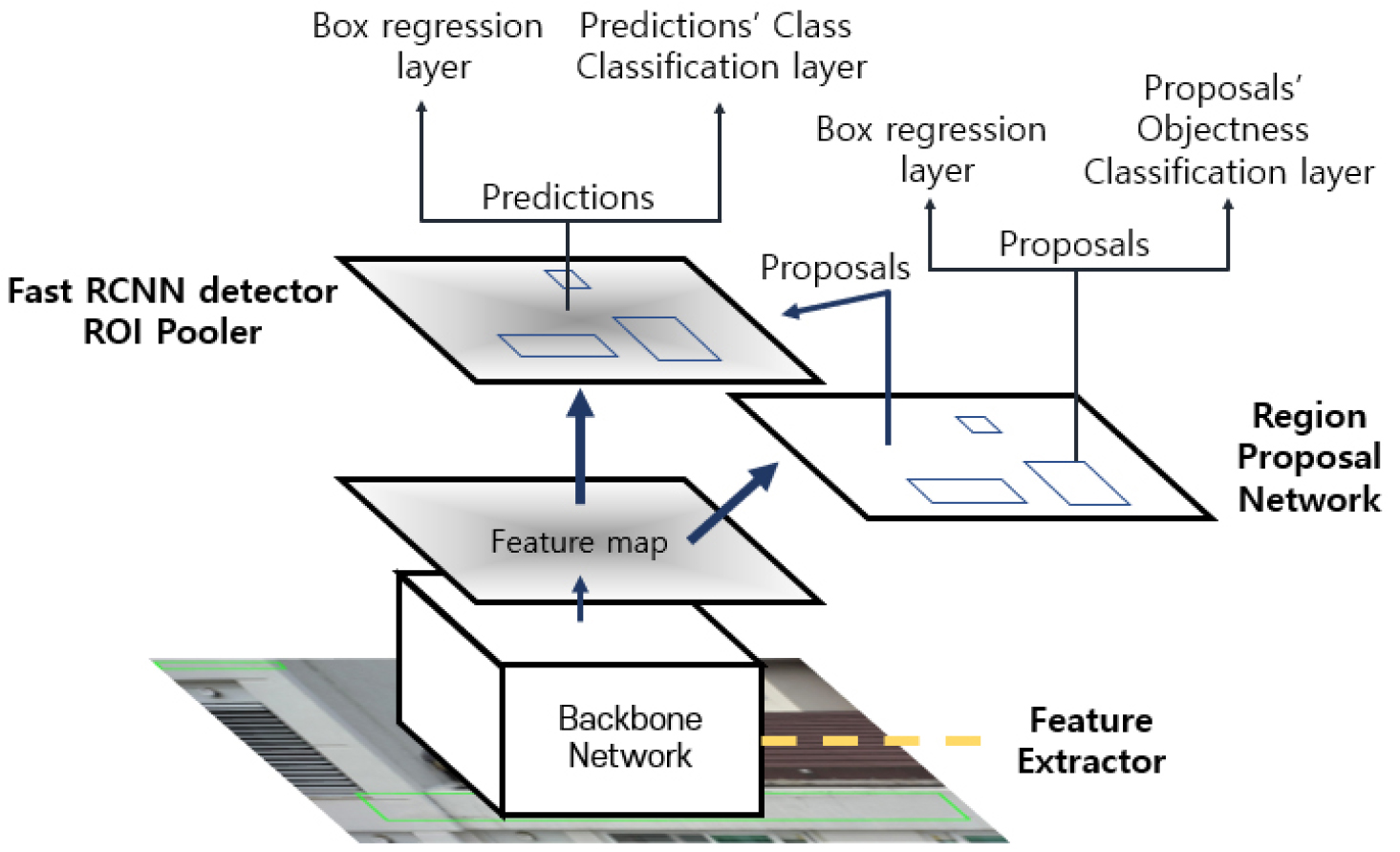
In addition, ResNet50 [28] was used as the backbone network that acts as a feature extractor in Faster R-CNN [27]. Because the backbone network serves to extract the features of an image, several CNN-based models can be used. Generally, features extracted through a CNN-based model contain higher-level information as the number of layers in the model increases. However, as the number of layers increases, the number of variables increases; thus, more data must be secured for better model training. ResNet learns the characteristics of an image using a residual learning method with a shortcut connection, and it exhibited superior performance in an image classification problem for the ImageNet dataset [28]. In addition, in an object detection task for the MS-COCO dataset, which aims at the same problem as this study, the experimental results when used as the backbone network of Faster R-CNN also showed high performance. Accordingly, in this study, ResNet was used as the backbone network of the basic model, and the ResNet50 model was used according to the number of samples in the dataset.

Accelerating the basic model (model compression)

Accelerating deep learning models is needed to compensate for physical limitations in the model training and inference through the trained model. Accelerating the model can derive the output nearly real time and accordingly it can be used in real life. A simple way to reduce the inference time of the model’s output is to use a lightweight model. A lightweight model mainly refers to a model with a small number of parameters and computations, and a model with fewer layers is usually lighter. However, when training on the same task using a lightweight model, performance degradation is likely to occur because the representation power of the model is different. As described earlier, performance degradation can be prevented in several ways. In this study, KD was used. The KD technique is a method that mimics the performance of a heavy model (model with a large number of layers) using the outputs of the heavy model for training a lightweight model. The heavy model is called the teacher network, whereas the lightweight model is called the student network. The teacher network starts in the already trained state, and in the output layer of the teacher network, logit, which is the value to which the activation function is not applied, is extracted and named as a soft label. In the classification task, the soft label is composed of a vector of probabilities that belong to each class, unlike the hard label used in the existing training. The soft loss calculated through the generated soft label is reflected in the loss previously used for the student network training. The KD method transfers the knowledge of the teacher network to the student network in this way. Equation 1 calculates the soft label in the classification task, where si is the probability of it belonging to class i, zi is a logit of the teacher network, and τ is the temperature:

Here, the variable τ represents the degree to which the probability distribution of the correct answer is smoothened so that it is easy to predict the output. The higher the value, the larger the value of the probability for the class close to 0. Accordingly, the probability distribution of the correct answer label becomes smoother. According to Chen et al. (2017) [23], for difficult tasks, such as object detection, the less smoothened labels results in a much better experimental results (τ=1). Therefore, in this study, τ=1 was used when calculating the classification loss.

The loss in the object detection task is largely classified into two categories: the loss calculated in the region proposal network (RPN) module, as depicted in Figure 1, and the loss calculated in the Fast R-CNN detector module. Each loss includes a loss from the box regression layer and a loss from the classification layer. In this study, KD was performed on the losses generated in the Fast R-CNN detector module, and through additional research, the KD method can be applied to the losses generated in the RPN module. In the following section, the details of the soft loss for the Fast R-CNN detector module are described.

Calculation of soft loss in the classification layer

The classification loss in the Fast R-CNN detector module is used to classify the objects existing in the box predicted by the network. The loss previously used in the classification layer is the cross-entropy loss, which is computed through Equation 2, where LhardCls is the cross-entropy loss (hard loss), S is the distribution of the predicted label by the student network, and P is the distribution of the ground-truth label (hard label):

According to Chen et al. (2017) [23], the soft loss for the classification task uses a class-weighted cross-entropy loss, which is used because of the label for the background class present in the soft label. Because most predicted objects belonging to the background class exist in the soft label, a data imbalance occurs between the foreground and background classes. By weighting the loss for the background class, choosing a foreground class other than the background makes the loss less. This method helps that the class of the box can be highly predicted as a foreground class other than the background class. Equation 3 computes the class-weighted cross entropy loss, where LsoftCls is the class-weighted cross-entropy loss (soft loss), S is the distribution of the predicted label by the student network, T is the distribution of the predicted label by the teacher network, and ωb is the weight for the background class:

Calculation of soft loss in the box regression layer

Basically, the loss in the box regression layer in the Faster R-CNN model uses the smooth L1 loss function. In this function, which is computed using Equation 4, β is a critical point where there is a change between L1 and L2 loss in the equation. In this study, the default value of 1 was used. In the equation, LhardReg is the smooth L1 loss (hard loss), xi,yi are the coordinates, and β is the threshold for changing the L1 and L2 loss.

Chen et al. (2017) [23] used the teacher-bounded regression loss for the soft loss for the box regression layer. This loss is used because the output derived from the box regression layer is an unbounded value. The unrestricted predicted value is also not limited to a range that may differ from the ground-truth label. Accordingly, if the soft label output from the teacher network is an incorrectly predicted label and the soft label is reflected in the training of the student network, then the difference from the actual label may be larger. Therefore, to prevent such an erroneous situation, the output of the box regression layer of the teacher network was not used as a direct target value for calculating the soft loss but was used as the upper bound of the output of the box regression layer of the student network. Equation 5 calculates the soft loss for the box regression layer of the lightweight model, where LsoftReg is the teacher-bounded regression loss (soft loss), Cs is the box coordinate vector predicted by the student network, Ct is the box coordinate vector predicted by the teacher network, C is the ground-truth box coordinate vector, and M is the margin:

In Equation 5, the hyperparameter called the margin increases as the upper bound of the value output from the box regression layer of the student network decreases. Lowering the upper bound may bring the output from the lightweight model closer to the coordinates of the actual box. In this study, the margins were determined through experiments. The total loss of the Faster R-CNN model can be expressed using the two soft losses mentioned earlier, which are the same as those in Equations 6, 7, 8, 9. In the equations, Ltotal is the total loss for training the student network, LRPN is the loss from the RPN module in the student network (equal to the teacher network’s loss), and Ldet is the loss from the Fast R-CNN detector module in the student network.

In these equations, α and κ are hyperparameters that indicate the degree to which soft loss is reflected in the box regression layer and the classification layer of the Fast R-CNN detector, respectively. These hyperparameters were determined through experiments. Through this process, it was possible to reduce the inference time and prevent performance degradation using a student network. The experimental results are presented in the next section.

Experiments and Results

Data collection and preprocessing

The input data used in this study are real-world images of the building façade, roof, and façade of an underground parking lot. The image data were obtained using drones and imaging devices. The purpose of this study is to accelerate multi-class defect detection in real-world image data through object detection model and KD method. Therefore, we constructed a branch to compute soft loss for high speed with object detection model, obtained real-world image data using drones and their combined imaging devices, and conducted experiments. In each image, defects were detected, which are used as objects in the object detection task. Objects in each image are represented by box coordinates, and each box is given a category ID according to the type of object. Four types of objects are used in this study, namely delamination, crack, peeled paint, and leakage, which are labeled as class 1, class 2, class 3, and class 4, respectively. The deep learning model used in this study aims to predict the coordinates of a box in which an object is located through an image and predicts the type of the corresponding box. To measure the generalization performance of the model, the data were divided into train, validation, and test datasets, and while training the model using the training dataset, the loss for the validation dataset was calculated to fine-tune the model’s hyperparameters. Table 1 shows the distribution of the data in each dataset. Before preprocessing, each image had a high resolution of 4,032×1,096 pixels. When the raw image of this size was used as the input data, the number of parameters in the deep learning model rapidly increased. Accordingly, the possibility of an overfitting problem inherently occurring in the deep learning model also increased. Because the overfitting problem significantly interferes with the model training, in this study, the size of the images was adjusted at the risk of information loss in the data. The size of each image was adjusted to 800×600 pixels. If the size was further reduced, then information on objects in the images is lost and cannot be distinguished with the naked eye.

Furthermore, because the number of layers and parameters of the basic model are large, the number of train datasets is insufficient to train the model. In deep learning, if the amount of data is insufficient, then the number of equations is smaller than the number of variables, and appropriate model training cannot be performed. Therefore, in this study, a data augmentation technique was used to increase the amount of data; random cropping and horizontal flipping were used. Horizontal flipping simply flipped the image around the vertical axis and was performed by the data loader in the model. The following is a description of the random cropping method, and Table 2 shows the structure of the training dataset changed using data proliferation.

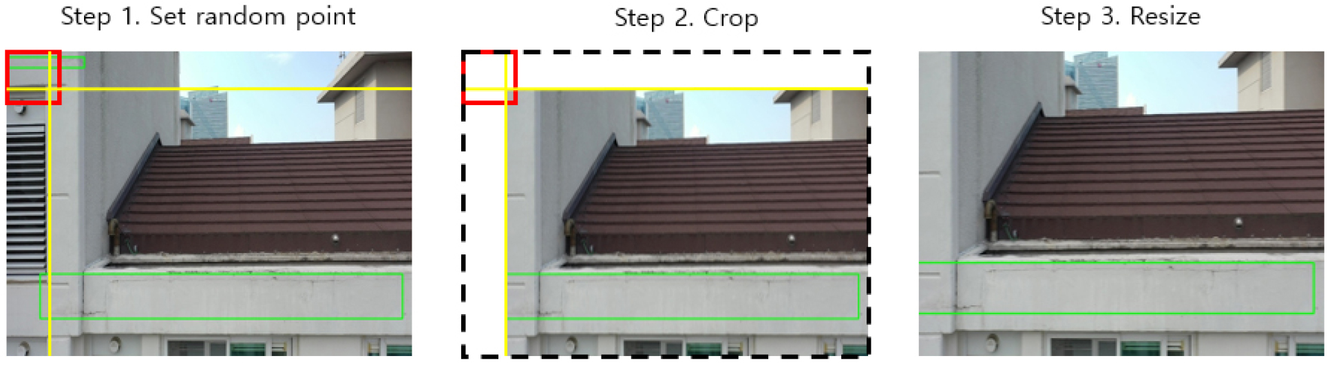
Random cropping is a data augmentation technique that cuts out a part of an existing image in the training dataset and uses it as a new image. There are several ways to crop an image. In this study, a method of cutting using random points was used. A zone that exists in an existing image was set, and a random point was set within that zone. The image was divided by drawing a vertical line and a horizontal line based on the set point, and the largest area was resized to the size of the existing image (800×600 pixels) to create new training data. If there was a ground-truth box that is cut together while cropping the image, a new object box coordinate was set using the size of the remaining area compared to the existing box. In this study, new coordinates were set when the cropped object box preserved more than 50% of the existing box area. By adding this to the train dataset, the amount of data that the model lacks in the training is compensated. Accordingly, the augmentation multiple can be adjusted by adjusting the number of random points. In this study, the data augmentation multiple was set to 20. Figure 2 shows a schematic of the random cutting method using random points.

Figure 2.

Random cropping process.

Experimental setting

As described earlier, in the experiment performed in this study, in addition to the hyperparameters used for basic training, hyperparameters necessary for calculating the soft loss were added. These hyperparameters are important factors in deriving an optimal model and were fine-tuned using the loss for the validation dataset. The optimization technique used to update the weight of the model is stochastic gradient descent (SGD) with momentum, which has the property of the existing SGD optimizer, and a feature that the direction of the previously updated weight was reflected to the next weight update [29]. The weight update is calculated using Equation (10), where ω is the weights, γ is the momentum, m is the momentum vector, and η is the learning rate:

The learning rate and momentum were set to 0.01 and 0.9, respectively, and the mini-batch size, the unit for updating the weight, was set to 8 according to the GPU performance used in the experiment.

Some hyperparameters were added while setting the prediction results of the teacher network as a soft label. The first hyperparameter is to filter out the prediction outputs of the teacher network. The prediction result was scored by the Faster R-CNN detector module. A score threshold for a prediction score is a hyperparameter that determines that the prediction result is used as a soft label for the student network only when the score exceeds the score threshold. This value determines the number and reliability of the soft labels. The second hyperparameter is to determine how the soft loss calculated through the aforementioned soft label is reflected in the student network’s training. Two losses were used to train the student network. One loss was generated by the hard label used to train the teacher network, and the other loss was generated by the prediction result of the teacher network (soft label). Determining the weights to properly mix the two losses and determine the degree to which the soft losses are reflected in the student network’s training.

In summary, the added hyperparameters are the score threshold as a criterion for extracting the soft label, weight α given to the soft loss in the classification layer, margin M as the criterion for extracting the soft loss in the regression layer, and weight κ given to the soft loss in the regression layer. These hyperparameters were determined experimentally, and their values were 0.7, 0.7, 10, and 0.5 in the order mentioned above.

Results and comparisons

The goal of this study is to speed up a deep learning model for detecting various types of defects on a building façade without the degradation of model performance. The performance of the model without speedup was compared with that of the speedup model. In addition, we compared the performance of the model trained by simply changing the backbone network to a more lightweight network and the model that was trained using the KD technique after weight reduction. The basic model (teacher network), that is, the Faster R-CNN model with ResNet50 as the backbone network, aims only for performance improvement. Because we used this model as a teacher network, we additionally used the feature pyramid network (FPN) to maximize its performance [30]. The high-speed model reduces the inference time using a more lightweight backbone network than the teacher network. This model uses MobileNetV2 [31] as the backbone network and does not add FPN for weight reduction. Table 3 shows the number of variables, number of operations in the Faster R-CNN model, and inference time based on GEFORCE RTX 2080Ti GPUs changed by reducing the weight of the central network.

As shown in Table 3, the inference time decreased by more than two times through the weight reduction. However, through the simple weight reduction, the performance of the model was significantly degraded. Figures 3 and 4 show the performance of the heavy model and that of the lightweight model in terms of the mean average precision (mAP) (intersection over union (IoU) = 0.5) and class, respectively.

Figure 3.

Performance of the teacher network (%) (ResNet50 backbone + FPN). x-axis : item separation (‘All’ is the average of all classes), y-axis : Average Precision (IoU=0.5).

Figure 4.

Performance of the student network (%) (MobileNetV2 backbone). x-axis : item separation (‘All’ is the average of all classes), y-axis : Average Precision (IoU=0.5).

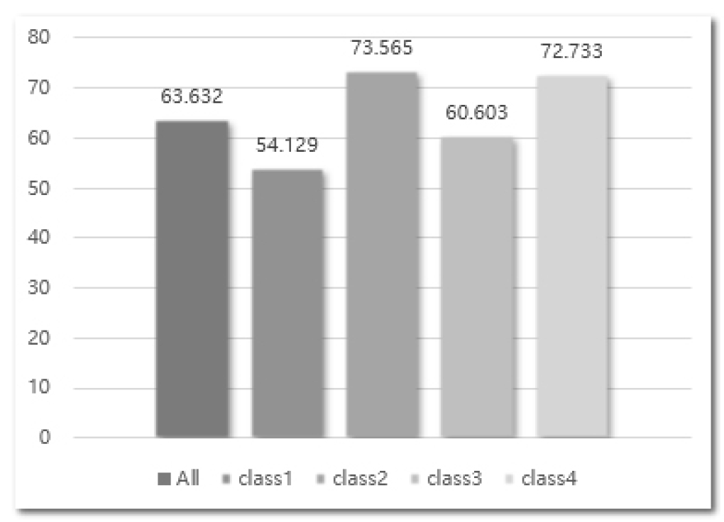
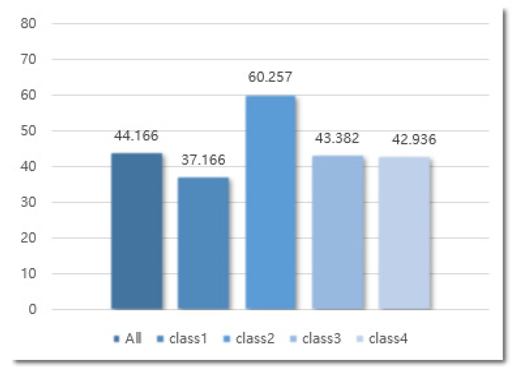
If the model used was simply lightweight and trained without using the KD technique, approximately 20% performance degradation occurred based on the mAP (IoU = 0.5). As mentioned above, as the model became lighter, the representation power decreased, and accordingly, the performance decreased. Therefore, for the Fast R-CNN detector module, a lightweight model was trained using the KD technique, and the results are presented in Figure 5. In addition, the precision-recall curve is shown in Figure 6.

Figure 5.

Performance of the student network with KD (%) (MobileNetV2 backbone). x-axis : item separation (‘All’ is the average of all classes), y-axis : Average Precision (IoU=0.5).

Figure 6.

Precision-recall curve for each class. x-axis : Recall, y-axis : Precision.

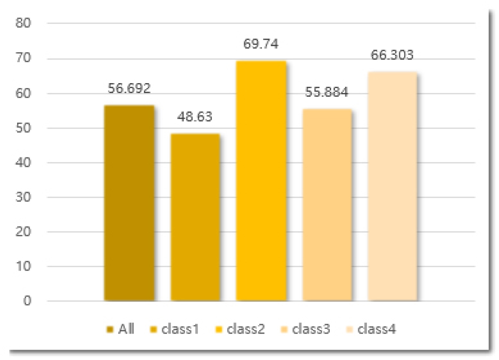
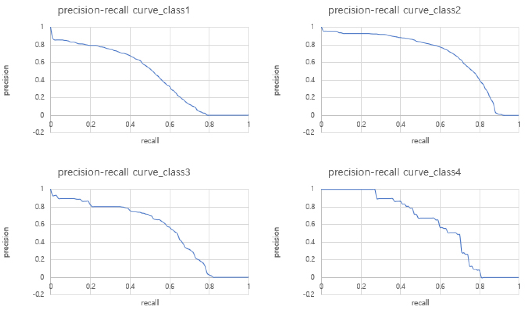
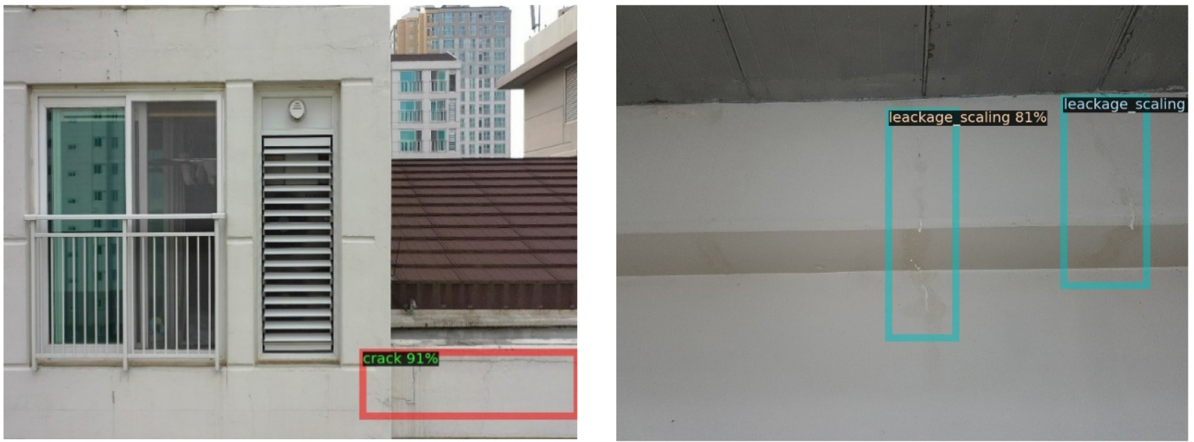
Figures 4 and 5 show an approximately 10% performance improvement based on mAP (IoU = 0.5). Through this method, it was possible to prove the effect of KD and to preserve efficiency and performance in the inference time. However, noting the difference in performance between Figures 3 and 5, there are still areas to be developed. Further research is needed for such areas to improve the defect detection in building façades in near real time. Figure 7 shows the sample images of the results inferred on the test dataset using a lightweight model with KD.

Figure 7.

Sample inferences using the student network with KD for the test dataset.

Conclusions

This paper is a study to accelerate the model for detecting defects present on the building façade. The purpose of this study is to photograph the residential building façade while detecting defects occurring on the building façade in real time. In this work, we used images of the residential building façade as input data for the model and considered them to be objects that want to detect defects present in the images. At this time, defects present in real building façade image data were detected using a model (Faster R-CNN) for object detection task, one of the major research fields using deep learning. As explained above, the model’s backbone network is intended to extract the high-level feature present in raw data. Because object detection tasks are a rather difficult problem, high-level features of data are required for high performance, and heavy networks are mainly used for this purpose. However, this violates the goal of detecting defects in real time because of the loss in terms of the inference time. In this work, we chose to use lighter network as backbone network among several methods to reduce the inference time. As described in “Experiments”, the use of this method results in a decrease in the detection performance of the model. Therefore, KD method was used as described in “Methodology” to prevent performance degradation of student network using light network as backbone network. The main contributions of this study are as follows.

1. We applied deep learning models and techniques to real-world image data to establish an automatic defect detection system that can check the building’s exterior walls in real time.

2. By using KD method, detection performance of models that occur during fastening process of deep learning model is prevented.

In the future, there is a need for research on improving the performance of teacher networks for detecting defects on building façades, accelerating models for object detection problems, and preventing performance degradation. To improve the performance of teacher networks, it is necessary to define the dataset more clearly and improve the detection model, among others. Moreover, to improve the performance of student networks that exhibit performance similar to those of teacher networks, we need to study other areas, such as fine-tuning hyperparameters for transferring the performance of the teacher network to the student network and developing methods to reflect knowledge in lightweight models. If research proceeds in this development direction, real-time automated detection of various types of defects will be possible.